神经网络与深度学习（邱锡鹏）编程练习 3 实验1 Logistic回归 pytorch

实验目标： 实现sigmoid的交叉熵损失函数(不使用tf内置的loss 函数)

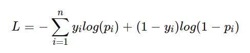
# 填空一，实现sigmoid的交叉熵损失函数(不使用内置的 loss 函数)
# loss_fn = nn.BCELoss()  # pytorch交叉熵损失函数
def loss_fn(label, pred): # 自定义 交叉熵损失函数
    epsilon = 1e-12
    cross_entropy = -label * torch.log(pred + epsilon) - (1. - label) * torch.log(1. - pred + epsilon)
    loss_mean = torch.mean(cross_entropy)
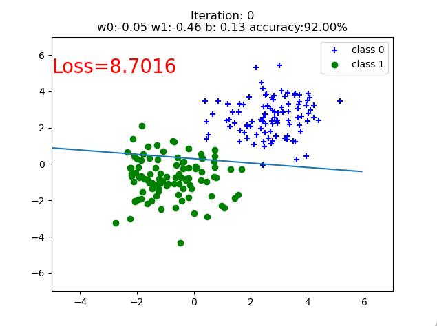
    return loss_mean

实验结果：

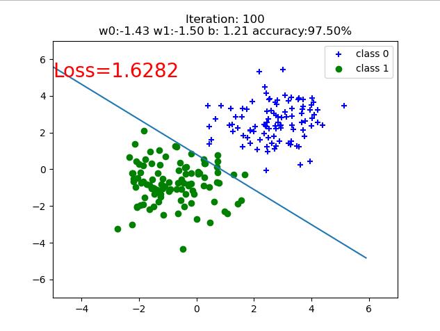
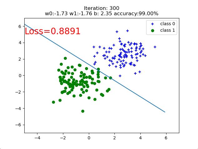
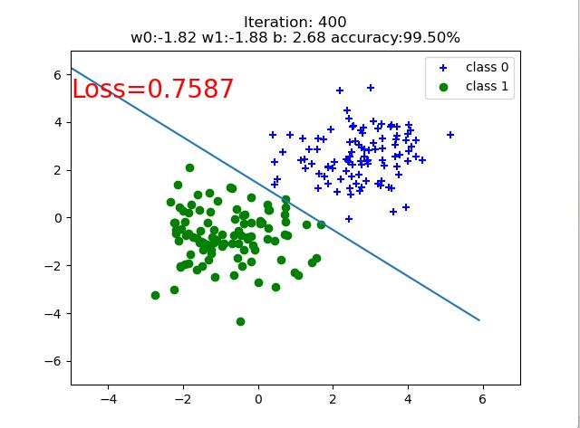
迭代400+之后，取得了较好的分类效果

过程可视化：

 

源代码：

import torch
import torch.nn as nn
import matplotlib.pyplot as plt
import numpy as np

# https://www.cnblogs.com/sakuraie/p/13341444.html
# https://www.cnblogs.com/douzujun/p/13296860.html

torch.manual_seed(10)

# ============================ step 1/5 生成数据 ============================
sample_nums = 100
mean_value = 1.7
bias = 1
n_data = torch.ones(sample_nums, 2)
x0 = torch.normal(mean_value * n_data, 1) + bias  # 类别0 数据 shape=(100, 2)
y0 = torch.zeros(sample_nums)  # 类别0 标签 shape=(100, 1)
x1 = torch.normal(-mean_value * n_data, 1) + bias  # 类别1 数据 shape=(100, 2)
y1 = torch.ones(sample_nums)  # 类别1 标签 shape=(100, 1)
train_x = torch.cat((x0, x1), 0)
train_y = torch.cat((y0, y1), 0)


# ============================ step 2/5 选择模型 ============================
class LR(nn.Module):
    def __init__(self):
        super(LR, self).__init__()
        self.features = nn.Linear(2, 1)
        self.sigmoid = nn.Sigmoid()

    def forward(self, x):
        x = self.features(x)
        x = self.sigmoid(x)
        return x


lr_net = LR()  # 实例化逻辑回归模型


# ============================ step 3/5 选择损失函数 ============================
# 填空一，实现sigmoid的交叉熵损失函数(不使用内置的 loss 函数)
# loss_fn = nn.BCELoss()  # pytorch交叉熵损失函数
def loss_fn(label, pred): # 自定义 交叉熵损失函数
    epsilon = 1e-12
    cross_entropy = -label * torch.log(pred + epsilon) - (1. - label) * torch.log(1. - pred + epsilon)
    loss_mean = torch.mean(cross_entropy)
    return loss_mean


# ============================ step 4/5 选择优化器   ============================
lr = 0.001  # 学习率
optimizer = torch.optim.SGD(lr_net.parameters(), lr=lr, momentum=0.9)

# ============================ step 5/5 模型训练 ============================
for iteration in range(501):
    y_pred = lr_net(train_x)  # 前向传播
    loss = loss_fn(y_pred.squeeze(), train_y)  # 计算 loss
    # print(loss)
    loss.requires_grad_(True)
    loss.backward()  # 反向传播
    optimizer.step()  # 更新参数
    optimizer.zero_grad()  # 清空梯度
    # 绘图
    if iteration % 100 == 0:
        mask = y_pred.ge(0.5).float().squeeze()  # 以0.5为阈值进行分类
        correct = (mask == train_y).sum()  # 计算正确预测的样本个数
        acc = correct.item() / train_y.size(0)  # 计算分类准确率

        plt.scatter(x0.data.numpy()[:, 0], x0.data.numpy()[:, 1], c='b', label='class 0', marker='+')
        plt.scatter(x1.data.numpy()[:, 0], x1.data.numpy()[:, 1], c='g', label='class 1', marker='o')

        w0, w1 = lr_net.features.weight[0]
        w0, w1 = float(w0.item()), float(w1.item())
        plot_b = float(lr_net.features.bias[0].item())
        plot_x = np.arange(-6, 6, 0.1)
        plot_y = (-w0 * plot_x - plot_b) / w1

        plt.xlim(-5, 7)
        plt.ylim(-7, 7)
        plt.plot(plot_x, plot_y)

        plt.text(-5, 5, 'Loss=%.4f' % loss.data.numpy(), fontdict={'size': 20, 'color': 'red'})
        print("iteration = ", iteration, "\tloss = ", loss.data.numpy())
        plt.title("Iteration: {}\nw0:{:.2f} w1:{:.2f} b: {:.2f} accuracy:{:.2%}".format(iteration, w0, w1, plot_b, acc))
        plt.legend()

        plt.show()
        plt.pause(0.5)

        if acc > 0.99:
            print("acc > 0.99")
            break

REF：

【邱希鹏】nndl-chap3-逻辑回归&softmax - douzujun - 博客园 (cnblogs.com)

 

 

 

 

 

Pytorch：通过pytorch实现逻辑回归 - 龙雪 - 博客园 (cnblogs.com)