神经网络与深度学习（邱锡鹏）编程练习 2 实验3 基函数回归（最小二乘法优化）

通过基函数对元素数据进行交换，从而将变量间的线性回归模型转换为非线性回归模型。

1. 最小二乘法 + 多项式基函数
2. 最小二乘法 + 高斯基函数

def multinomial_basis(x, feature_num=10):
    x = np.expand_dims(x, axis=1) # shape(N, 1)
    feat = [x]
    for i in range(2, feature_num+1):
        feat.append(x**i)
    ret = np.concatenate(feat, axis=1)
    return ret

def gaussian_basis(x, feature_num=10):
    centers = np.linspace(0, 25, feature_num)
    width = 1.0 * (centers[1] - centers[0])
    x = np.expand_dims(x, axis=1)
    x = np.concatenate([x]*feature_num, axis=1)
    
    out = (x-centers)/width
    ret = np.exp(-0.5 * out ** 2)
    return ret

实验结果：

 

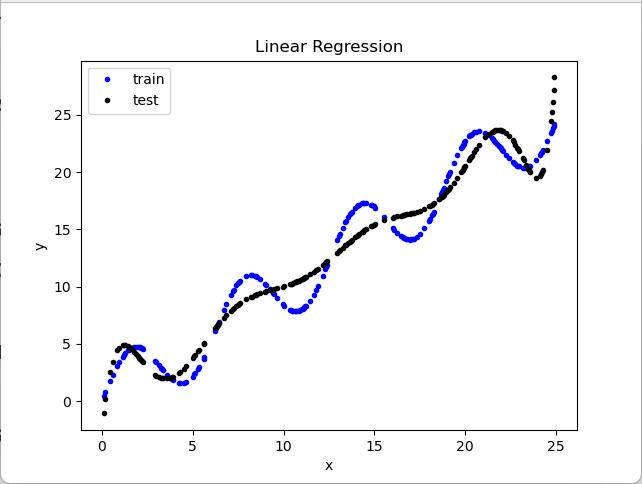
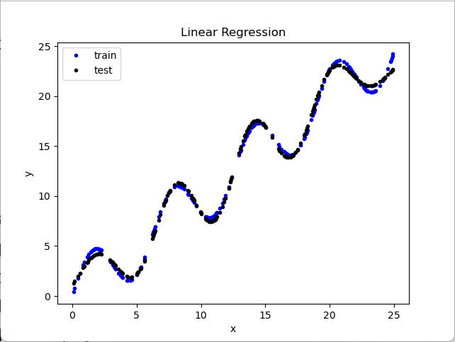
实验结果分析：

多项式回归（多项式基函数）比线性回归更好的拟合了数据

高斯基函数拟合效果比多项式基函数拟合效果更好

 

多项式基函数源代码：

查看代码

import numpy as np
import matplotlib.pyplot as plt


def load_data(filename):  # 载入数据
    xys = []
    with open(filename, 'r') as f:
        for line in f:
            xys.append(map(float, line.strip().split()))
        xs, ys = zip(*xys)
        return np.asarray(xs), np.asarray(ys)


def multinomial_basis(x, feature_num=10):
    x = np.expand_dims(x, axis=1)  # shape(N, 1)
    feat = [x]
    for i in range(2, feature_num + 1):
        feat.append(x ** i)
    ret = np.concatenate(feat, axis=1)
    return ret


def main(x_train, y_train):  # 训练模型，并返回从x到y的映射。
    basis_func = multinomial_basis  # shape(N, 1)的函数
    phi0 = np.expand_dims(np.ones_like(x_train), axis=1)  # shape(N,1)大小的全1 array
    phi1 = basis_func(x_train)  # 将x_train的shape转换为(N, 1)
    phi = np.concatenate([phi0, phi1], axis=1)  # phi.shape=(300,2) phi是增广特征向量的转置
    print("phi shape = ", phi.shape)
    # 使用最小二乘法优化w
    w = np.dot(np.linalg.pinv(phi), y_train)  # np.linalg.pinv(phi)求phi的伪逆矩阵(phi不是列满秩) w.shape=[2,1]
    print("参数 w = ", w)

    def f(x):
        phi0 = np.expand_dims(np.ones_like(x), axis=1)
        phi1 = basis_func(x)
        phi = np.concatenate([phi0, phi1], axis=1)
        y = np.dot(phi, w)  # 矩阵乘法
        return y

    return f


def evaluate(ys, ys_pred):  # 评估模型
    std = np.sqrt(np.mean(np.abs(ys - ys_pred) ** 2))
    return std


if __name__ == '__main__':  # 程序主入口（建议不要改动以下函数的接口）
    train_file = 'train.txt'
    test_file = 'test.txt'
    # 载入数据
    x_train, y_train = load_data(train_file)
    x_test, y_test = load_data(test_file)
    print("x_train shape:", x_train.shape)
    print("x_test shape:", x_test.shape)

    # 训练模型，返回一个函数f()使得 y = f(x)
    f = main(x_train, y_train)

    y_train_pred = f(x_train)  # 训练集 预测值
    std = evaluate(y_train, y_train_pred) # 使用训练集评估模型
    print('训练集 预测值与真实值的标准差：{:.1f}'.format(std))

    y_test_pred = f(x_test)  # 测试集 预测值
    std = evaluate(y_test, y_test_pred)  # 使用测试集评估模型
    print('测试集 预测值与真实值的标准差：{:.1f}'.format(std))

    # 显示结果
    # plt.plot(x_train, y_train, 'r.')  # 训练集
    plt.plot(x_test, y_test, 'b.')  # 测试集
    plt.plot(x_test, y_test_pred, 'k.')  # 测试集 的 预测值
    plt.xlabel('x')
    plt.ylabel('y')
    plt.title('Linear Regression')
    plt.legend(['train', 'test', 'pred'])
    plt.show()

高斯基函数源代码：

查看代码

import numpy as np
import matplotlib.pyplot as plt


def load_data(filename):  # 载入数据
    xys = []
    with open(filename, 'r') as f:
        for line in f:
            xys.append(map(float, line.strip().split()))
        xs, ys = zip(*xys)
        return np.asarray(xs), np.asarray(ys)


def gaussian_basis(x, feature_num=10):
    centers = np.linspace(0, 25, feature_num)
    width = 1.0 * (centers[1] - centers[0])
    x = np.expand_dims(x, axis=1)
    x = np.concatenate([x] * feature_num, axis=1)

    out = (x - centers) / width
    ret = np.exp(-0.5 * out ** 2)
    return ret


def main(x_train, y_train):  # 训练模型，并返回从x到y的映射。
    basis_func = gaussian_basis  # shape(N, 1)的函数
    phi0 = np.expand_dims(np.ones_like(x_train), axis=1)  # shape(N,1)大小的全1 array
    phi1 = basis_func(x_train)  # 将x_train的shape转换为(N, 1)
    phi = np.concatenate([phi0, phi1], axis=1)  # phi.shape=(300,2) phi是增广特征向量的转置
    print("phi shape = ", phi.shape)
    # 使用最小二乘法优化w
    w = np.dot(np.linalg.pinv(phi), y_train)  # np.linalg.pinv(phi)求phi的伪逆矩阵(phi不是列满秩) w.shape=[2,1]
    print("参数 w = ", w)

    def f(x):
        phi0 = np.expand_dims(np.ones_like(x), axis=1)
        phi1 = basis_func(x)
        phi = np.concatenate([phi0, phi1], axis=1)
        y = np.dot(phi, w)  # 矩阵乘法
        return y

    return f


def evaluate(ys, ys_pred):  # 评估模型
    std = np.sqrt(np.mean(np.abs(ys - ys_pred) ** 2))
    return std


if __name__ == '__main__':  # 程序主入口（建议不要改动以下函数的接口）
    train_file = 'train.txt'
    test_file = 'test.txt'
    # 载入数据
    x_train, y_train = load_data(train_file)
    x_test, y_test = load_data(test_file)
    print("x_train shape:", x_train.shape)
    print("x_test shape:", x_test.shape)

    # 训练模型，返回一个函数f()使得 y = f(x)
    f = main(x_train, y_train)

    y_train_pred = f(x_train)  # 训练集 预测值
    std = evaluate(y_train, y_train_pred) # 使用训练集评估模型
    print('训练集 预测值与真实值的标准差：{:.1f}'.format(std))

    y_test_pred = f(x_test)  # 测试集 预测值
    std = evaluate(y_test, y_test_pred)  # 使用测试集评估模型
    print('测试集 预测值与真实值的标准差：{:.1f}'.format(std))

    # 显示结果
    # plt.plot(x_train, y_train, 'r.')  # 训练集
    plt.plot(x_test, y_test, 'b.')  # 测试集
    plt.plot(x_test, y_test_pred, 'k.')  # 测试集 的 预测值
    plt.xlabel('x')
    plt.ylabel('y')
    plt.title('Linear Regression')
    plt.legend(['train', 'test', 'pred'])
    plt.show()