神经网络与深度学习（邱锡鹏）编程练习 2 实验2 线性回归的参数优化 - 梯度下降法

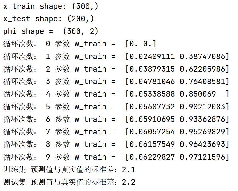
实验结果：

源代码：

import numpy as np
import matplotlib.pyplot as plt


def load_data(filename):  # 载入数据
    xys = []
    with open(filename, 'r') as f:
        for line in f:
            xys.append(map(float, line.strip().split()))
        xs, ys = zip(*xys)
        return np.asarray(xs), np.asarray(ys)


def identity_basis(x):
    ret = np.expand_dims(x, axis=1)  # x原先为1维（只有轴axis=0）的数组，使用expand_dims扩展出1维（扩展出轴axis=1）
    return ret


def main(x_train, y_train):  # 训练模型，并返回从x到y的映射。
    basis_func = identity_basis  # shape(N, 1)的函数
    phi0 = np.expand_dims(np.ones_like(x_train), axis=1)  # shape(N,1)大小的全1 array
    phi1 = basis_func(x_train)  # 将x_train的shape转换为(N, 1)
    phi = np.concatenate([phi0, phi1], axis=1)  # phi.shape=(300,2) phi是增广特征向量的转置
    print("phi shape = ", phi.shape)

    # 梯度下降法 优化w
    def gradient(phi_grad, y, w_init, lr=0.001, step_num=10):  # lr 学习率; step_num 迭代次数
        w_train = w_init
        for i in range(step_num):
            print("循环次数：", i, "参数 w_train = ", w_train)
            grad = phi_grad.T.dot(phi_grad.dot(w_train) - y) * 2.0 / len(phi_grad)  # 计算梯度
            w_train = w_train - lr * grad  # 更新 w
        return w_train

    init_theta = np.zeros(phi.shape[1])
    w = gradient(phi, y_train, init_theta)

    def f(x):
        phi0 = np.expand_dims(np.ones_like(x), axis=1)
        phi1 = basis_func(x)
        phi = np.concatenate([phi0, phi1], axis=1)
        y = np.dot(phi, w)  # 矩阵乘法
        return y

    return f


def evaluate(ys, ys_pred):  # 评估模型
    std = np.sqrt(np.mean(np.abs(ys - ys_pred) ** 2))
    return std


if __name__ == '__main__':  # 程序主入口（建议不要改动以下函数的接口）
    train_file = 'train.txt'
    test_file = 'test.txt'
    # 载入数据
    x_train, y_train = load_data(train_file)
    x_test, y_test = load_data(test_file)
    print("x_train shape:", x_train.shape)
    print("x_test shape:", x_test.shape)

    # 训练模型，返回一个函数f()使得 y = f(x)
    f = main(x_train, y_train)

    y_train_pred = f(x_train)  # 训练集 预测值
    std = evaluate(y_train, y_train_pred)  # 使用训练集评估模型
    print('训练集 预测值与真实值的标准差：{:.1f}'.format(std))

    y_test_pred = f(x_test)  # 测试集 预测值
    std = evaluate(y_test, y_test_pred)  # 使用测试集评估模型
    print('测试集 预测值与真实值的标准差：{:.1f}'.format(std))

    # 显示结果
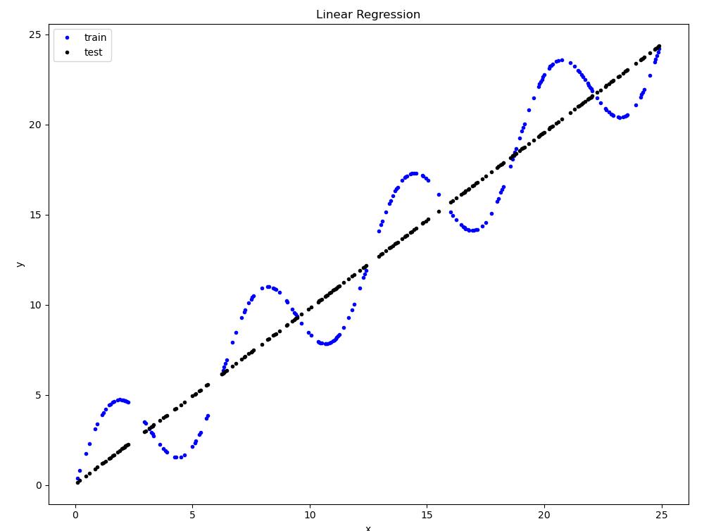
    # plt.plot(x_train, y_train, 'r.')  # 训练集
    plt.plot(x_test, y_test, 'b.')  # 测试集
    plt.plot(x_test, y_test_pred, 'k.')  # 测试集 的 预测值
    plt.xlabel('x')
    plt.ylabel('y')
    plt.title('Linear Regression')
    plt.legend(['train', 'test', 'pred'])
    plt.show()

 

REF：【邱希鹏】nndl-chap2-linear_regression - douzujun - 博客园 (cnblogs.com)