

一、用神经网络Sequential(序贯模型)搭建
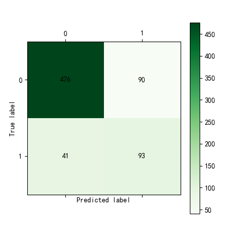
1 2 3 4 5 6 7 8 9 10 11 12 13 14 15 16 17 18 19 20 21 22 23 24 25 26 27 28 29 30 31 32 33 34 35 36 37 38 39 40 41 42 43 | import pandas as pdimport numpy as np#导入划分数据集函数from sklearn.model_selection import train_test_split#读取数据datafile = 'E:\\桌面\\作业\py\\bankloan.xls'#文件路径data = pd.read_excel(datafile)x = data.iloc[:,:8]y = data.iloc[:,8]#划分数据集x_train, x_test, y_train, y_test = train_test_split(x, y, test_size=0.2, random_state=100)#导入模型和函数from keras.models import Sequentialfrom keras.layers import Dense,Dropout#导入指标from keras.metrics import BinaryAccuracy#导入时间库计时import timestart_time = time.time()#-------------------------------------------------------#model = Sequential()model.add(Dense(input_dim=8,units=800,activation='relu'))#激活函数relumodel.add(Dropout(0.5))#防止过拟合的掉落函数model.add(Dense(input_dim=800,units=400,activation='relu'))model.add(Dropout(0.5))model.add(Dense(input_dim=400,units=1,activation='sigmoid'))model.compile(loss='binary_crossentropy', optimizer='adam',metrics=[BinaryAccuracy()])model.fit(x_train,y_train,epochs=100,batch_size=128)loss,binary_accuracy = model.evaluate(x,y,batch_size=128)#--------------------------------------------------------#end_time = time.time()run_time = end_time-start_time#运行时间print('模型运行时间:{}'.format(run_time))print('模型损失值:{}'.format(loss))print('模型精度:{}'.format(binary_accuracy))yp = model.predict(x).reshape(len(y))yp = np.around(yp,0).astype(int) #转换为整型from cm_plot import * # 导入自行编写的混淆矩阵可视化函数cm_plot(y,yp).show() # 显示混淆矩阵可视化结果 |
cm_plot函数:
1 2 3 4 5 6 7 8 9 10 11 12 13 14 15 16 17 18 | #-*- coding: utf-8 -*-def cm_plot(y, yp): from sklearn.metrics import confusion_matrix #导入混淆矩阵函数 cm = confusion_matrix(y, yp) #混淆矩阵 import matplotlib.pyplot as plt #导入作图库 plt.matshow(cm, cmap=plt.cm.Greens) #画混淆矩阵图,配色风格使用cm.Greens,更多风格请参考官网。 plt.colorbar() #颜色标签 for x in range(len(cm)): #数据标签 for y in range(len(cm)): plt.annotate(cm[x,y], xy=(x, y), horizontalalignment='center', verticalalignment='center') plt.ylabel('True label') #坐标轴标签 plt.xlabel('Predicted label') #坐标轴标签 return plt |
结果
二、用机器学习相关算法搭建
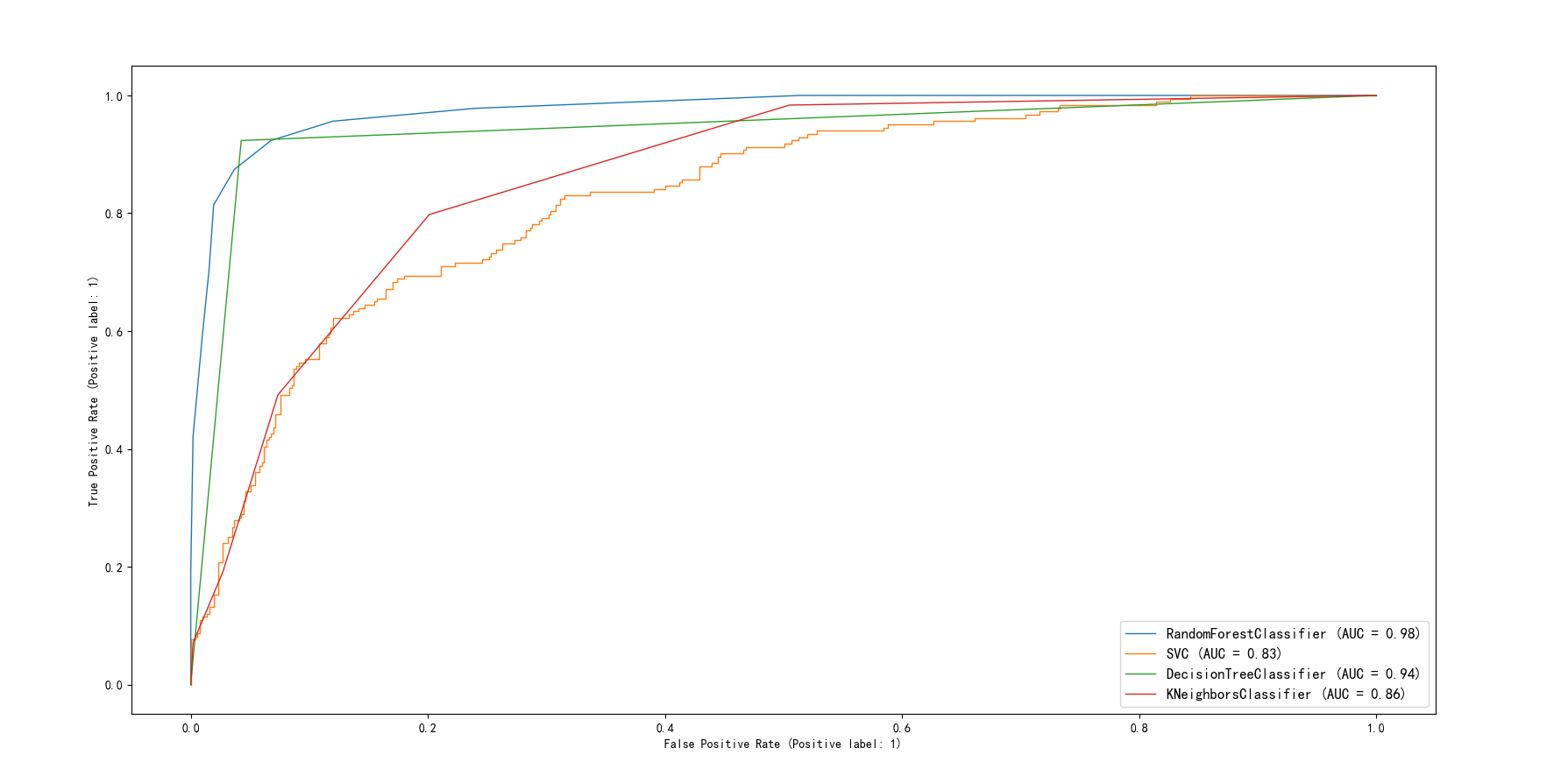
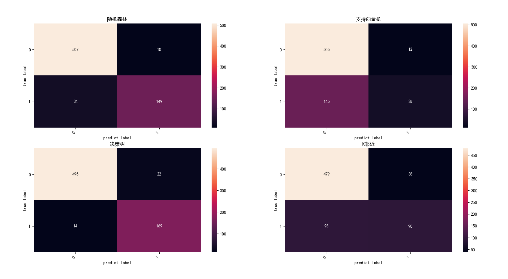
1、支持向量机(SVM)、随机森林、决策树、KNN(K邻近)
1 2 3 4 5 6 7 8 9 10 11 12 13 14 15 16 17 18 19 20 21 22 23 24 25 26 27 28 29 30 31 32 33 34 35 36 37 38 39 40 41 42 43 44 45 46 47 48 49 50 51 52 53 54 55 56 57 58 59 60 61 62 63 64 65 66 67 68 69 70 71 72 73 74 75 76 77 78 79 80 81 82 83 84 85 86 87 88 89 90 91 92 93 94 95 96 97 98 99 100 101 102 103 104 105 106 107 108 109 110 111 112 113 114 115 116 117 118 119 120 121 122 123 124 125 126 127 128 129 130 131 132 | # -*- coding: utf-8 -*-"""Created on Sun Mar 27 19:33:58 2022@author: 86183"""import pandas as pdimport timeimport numpy as npimport seaborn as snsimport matplotlib.pyplot as plt from sklearn.model_selection import train_test_splitfrom sklearn.tree import DecisionTreeClassifier as DTCfrom sklearn.ensemble import RandomForestClassifier as RFCfrom sklearn import svmfrom sklearn import treefrom sklearn.metrics import confusion_matrixfrom sklearn.metrics import accuracy_scorefrom sklearn.metrics import roc_curve, aucfrom sklearn.neighbors import KNeighborsClassifier as KNN#导入plot_roc_curve,roc_curve和roc_auc_score模块from sklearn.metrics import plot_roc_curve,roc_curve,auc,roc_auc_scorefilePath = 'E:/桌面/作业\py/bankloan.xls'data = pd.read_excel(filePath)x = data.iloc[:,:8]y = data.iloc[:,8]x_train, x_test, y_train, y_test = train_test_split(x, y, test_size=0.2, random_state=100)#模型svm_clf = svm.SVC()#支持向量机dtc_clf = DTC(criterion='entropy')#决策树rfc_clf = RFC(n_estimators=10)#随机森林knn_clf = KNN()#K邻近#训练knn_clf.fit(x_train,y_train)rfc_clf.fit(x_train,y_train)dtc_clf.fit(x_train,y_train)svm_clf.fit(x_train, y_train)#ROC曲线比较fig,ax = plt.subplots(figsize=(12,10))rfc_roc = plot_roc_curve(estimator=rfc_clf, X=x, y=y, ax=ax, linewidth=1)svm_roc = plot_roc_curve(estimator=svm_clf, X=x, y=y, ax=ax, linewidth=1)dtc_roc = plot_roc_curve(estimator=dtc_clf, X=x, y=y, ax=ax, linewidth=1)knn_roc = plot_roc_curve(estimator=knn_clf, X=x, y=y, ax=ax, linewidth=1)ax.legend(fontsize=12)plt.show()#模型评价rfc_yp = rfc_clf.predict(x)rfc_score = accuracy_score(y, rfc_yp)svm_yp = svm_clf.predict(x)svm_score = accuracy_score(y, svm_yp)dtc_yp = dtc_clf.predict(x)dtc_score = accuracy_score(y, dtc_yp)knn_yp = knn_clf.predict(x)knn_score = accuracy_score(y, knn_yp)score = {"随机森林得分":rfc_score,"支持向量机得分":svm_score,"决策树得分":dtc_score,"K邻近得分":knn_score}score = sorted(score.items(),key = lambda score:score[0],reverse=True)print(pd.DataFrame(score))#中文标签、负号正常显示plt.rcParams['font.sans-serif'] = ['SimHei']plt.rcParams['axes.unicode_minus'] = False#绘制混淆矩阵figure = plt.subplots(figsize=(12,10))plt.subplot(2,2,1)plt.title('随机森林')rfc_cm = confusion_matrix(y, rfc_yp)heatmap = sns.heatmap(rfc_cm, annot=True, fmt='d')heatmap.yaxis.set_ticklabels(heatmap.yaxis.get_ticklabels(), rotation=0, ha='right')heatmap.xaxis.set_ticklabels(heatmap.xaxis.get_ticklabels(), rotation=45, ha='right')plt.ylabel("true label")plt.xlabel("predict label")plt.subplot(2,2,2)plt.title('支持向量机')svm_cm = confusion_matrix(y, svm_yp)heatmap = sns.heatmap(svm_cm, annot=True, fmt='d')heatmap.yaxis.set_ticklabels(heatmap.yaxis.get_ticklabels(), rotation=0, ha='right')heatmap.xaxis.set_ticklabels(heatmap.xaxis.get_ticklabels(), rotation=45, ha='right')plt.ylabel("true label")plt.xlabel("predict label")plt.subplot(2,2,3)plt.title('决策树')dtc_cm = confusion_matrix(y, dtc_yp)heatmap = sns.heatmap(dtc_cm, annot=True, fmt='d')heatmap.yaxis.set_ticklabels(heatmap.yaxis.get_ticklabels(), rotation=0, ha='right')heatmap.xaxis.set_ticklabels(heatmap.xaxis.get_ticklabels(), rotation=45, ha='right')plt.ylabel("true label")plt.xlabel("predict label")plt.subplot(2,2,4)plt.title('K邻近')knn_cm = confusion_matrix(y, knn_yp)heatmap = sns.heatmap(knn_cm, annot=True, fmt='d')heatmap.yaxis.set_ticklabels(heatmap.yaxis.get_ticklabels(), rotation=0, ha='right')heatmap.xaxis.set_ticklabels(heatmap.xaxis.get_ticklabels(), rotation=45, ha='right')plt.ylabel("true label")plt.xlabel("predict label")plt.show()#画出决策树import pandas as pdimport osos.environ["PATH"] += os.pathsep + 'D:/软件下载安装/Graphviz/bin'from sklearn.tree import export_graphvizx = pd.DataFrame(x)with open(r"E:/桌面/作业/py/banklodan_tree.dot", 'w') as f: export_graphviz(dtc_clf, feature_names = x.columns, out_file = f) f.close() from IPython.display import Image from sklearn import treeimport pydotplus dot_data = tree.export_graphviz(dtc_clf, out_file=None, #regr_1 是对应分类器 feature_names=x.columns, #对应特征的名字 class_names= ['不违约','违约'], #对应类别的名字 filled=True, rounded=True, special_characters=True) 让graphviz显示中文用"MicrosoftYaHei"代替'helvetica'graph = pydotplus.graph_from_dot_data(dot_data.replace('helvetica',"MicrosoftYaHei")) graph.write_png('C:/Users/86188/Desktop/Python数据挖掘与数据分析/My work/tmp/banklodan_tree.png') #保存图像Image(graph.create_png()) |
ROC曲线:
混淆矩阵:
得分:
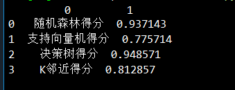
综上:决策树和随机森林的效果最好,总体上都比神经网络的要好


【推荐】国内首个AI IDE,深度理解中文开发场景,立即下载体验Trae
【推荐】编程新体验,更懂你的AI,立即体验豆包MarsCode编程助手
【推荐】抖音旗下AI助手豆包,你的智能百科全书,全免费不限次数
【推荐】轻量又高性能的 SSH 工具 IShell:AI 加持,快人一步
· TypeScript + Deepseek 打造卜卦网站:技术与玄学的结合
· Manus的开源复刻OpenManus初探
· AI 智能体引爆开源社区「GitHub 热点速览」
· 三行代码完成国际化适配,妙~啊~
· .NET Core 中如何实现缓存的预热?