A Neural Probabilistic Language Model_论文阅读及代码复现pytorch版
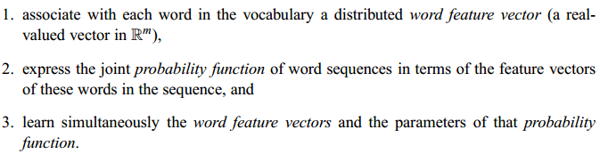
针对的问题:
- 维度灾难。常见于在要对许多离散随机变量之间的联合分布进行建模的情况下;
- 如何考虑到超过1个或2个单词的上下文;
- 如何考虑到单词之间的相似性。
- 引入分布式表示,通过使得相似上下文和相似句子中词的向量彼此接近,因此得到泛化性。分布式表示(Distributed representation)最早是 Hinton 在 1986 年的论文《Learning distributed representations of concepts》中提出的。Distributed representation 用来表示词,通常被称为“Word Representation”或“Word Embedding”,中文俗称“词向量”或“词嵌入”。
所提方法的思想:
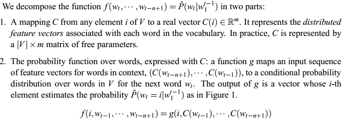
模型:

-
- 目标:上图中最下方的wt-n+1,...,wt-2,wt-1就是前n-1个单词,现在根据这已知的n-1个单词预测下一个单词wt。
- 模型一共三层
- 第一层是映射层,将n个单词映射为对应word embeddings的拼接,其实这一层就是MLP的输入层;
- 第二层是隐藏层,激活函数用tanh;
- 第三层是输出层,因为是语言模型,需要根据前n个单词预测下一个单词,所以是一个多分类器,用softmax。
- 整个模型最大的计算量集中在最后一层上,因为一般来说词汇表都很大,需要计算每个单词的条件概率,是整个模型的计算瓶颈。
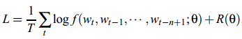
- 最大正则化对数似然函数:
-
-
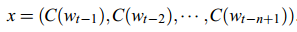
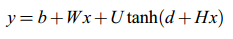
x是第一层输入层的激活向量,来自矩阵C的输入词特征的连接:
-
-
- 第二层(隐藏层)直接用d+Hx计算得到。
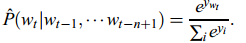
- 第三层(输出层)一共有|V|个节点,每个节点yi表示下一个单词i的未归一化log概率。最后使用softmax函数将输出值y归一化成概率,最终y的计算公式如下:
-
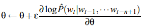
- 通过SGD进行参数更新
- 参数介绍:
- h be the number of hidden units
- m the number of features associated with each word
- b the output biases
- d the hidden layer biases
- U the hidden-to-output weights (a |V|×h matrix)
- H the hidden layer weights (a h × (n − 1)m matrix)
- W the word features to output weights(a |V| × (n − 1)m matrix)
- C the word features(a |V|×m matrix)
- 通过SGD进行参数更新:
代码:来自https://github.com/graykode/nlp-tutorial/tree/master/1-1.NNLM
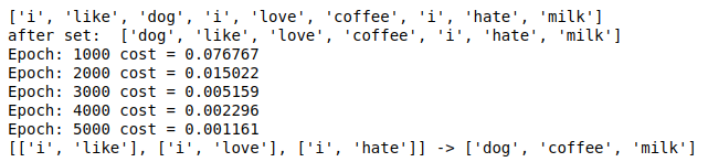
# code by Tae Hwan Jung @graykode
import numpy as np
import torch
import torch.nn as nn
import torch.optim as optim
from torch.autograd import Variable

dtype = torch.FloatTensor

sentences = [ "i like dog", "i love coffee", "i hate milk"]

word_list = " ".join(sentences).split()  #制作词汇表
print(word_list)
word_list = list(set(word_list))  #去重
print("after set: ",word_list)
word_dict = {w: i for i, w in enumerate(word_list)}  #每个单词对应的索引
number_dict = {i: w for i, w in enumerate(word_list)}  #每个索引对应的单词
n_class = len(word_dict) # 单词总数

# NNLM Parameter
n_step = 2 #  根据前两个单词预测第3个单词
n_hidden = 2 # h 隐藏层神经元的个数
m = 2 # m 词向量的维度

# 由于pytorch中输入的数据是以batch小批量进行输入的,下面的函数就是将原始数据以一个batch为基本单位喂给模型
def make_batch(sentences):
    input_batch = []
    target_batch = []

    for sen in sentences:
        word = sen.split()
        input = [word_dict[n] for n in word[:-1]]
        target = word_dict[word[-1]]

        input_batch.append(input)
        target_batch.append(target)

    return input_batch, target_batch

# Model
class NNLM(nn.Module):
    def __init__(self):
        super(NNLM, self).__init__()
        self.C = nn.Embedding(n_class, m)
        self.H = nn.Parameter(torch.randn(n_step * m, n_hidden).type(dtype))
        self.W = nn.Parameter(torch.randn(n_step * m, n_class).type(dtype))
        self.d = nn.Parameter(torch.randn(n_hidden).type(dtype))
        self.U = nn.Parameter(torch.randn(n_hidden, n_class).type(dtype))
        self.b = nn.Parameter(torch.randn(n_class).type(dtype))

    def forward(self, X):
        X = self.C(X)
        X = X.view(-1, n_step * m) # [batch_size, n_step * n_class]
        tanh = torch.tanh(self.d + torch.mm(X, self.H)) # [batch_size, n_hidden]
        output = self.b + torch.mm(X, self.W) + torch.mm(tanh, self.U) # [batch_size, n_class]
        return output

model = NNLM()

criterion = nn.CrossEntropyLoss()
optimizer = optim.Adam(model.parameters(), lr=0.001)

input_batch, target_batch = make_batch(sentences)
input_batch = Variable(torch.LongTensor(input_batch))
target_batch = Variable(torch.LongTensor(target_batch))

# 对于每个batch大都执行了以下这样的操作,可理解为梯度下降法
# Training
for epoch in range(5000):

    optimizer.zero_grad()  # 把梯度置零,也就是把loss关于weight的导数变成0.

    output = model(input_batch)  #前向传播求出预测的值

    # output : [batch_size, n_class], target_batch : [batch_size] (LongTensor, not one-hot)
    loss = criterion(output, target_batch)  # 求loss
    if (epoch + 1)%1000 == 0:
        print('Epoch:', '%04d' % (epoch + 1), 'cost =', '{:.6f}'.format(loss))

    loss.backward()  # 反向传播求梯度
    optimizer.step()  # 更新所有参数

# 为什么调用backward()函数之前都要将梯度清零
# 因为如果梯度不清零,pytorch中会将上次计算的梯度和本次计算的梯度累加。
# 这样逻辑的好处--当我们的硬件限制不能使用更大的bachsize时,使用多次计算较小的bachsize的梯度平均值来代替,更方便,
# 坏处--每次都要清零梯度

# Predict
predict = model(input_batch).data.max(1, keepdim=True)[1]

# Test
print([sen.split()[:2] for sen in sentences], '->', [number_dict[n.item()] for n in predict.squeeze()])
结果:

 浙公网安备 33010602011771号