吴恩达深度学习第四课第一周编程作业_Convolutional Neural Networks: Application

Convolutional Neural Networks: Application 卷积神经网络应用

本文参考了深度学习吴恩达小迷弟的文章，链接：https://blog.csdn.net/weixin_47440593/article/details/107938235

欢迎来到课程4的第二次作业!在这个笔记本里，你会:

·实现在实现TensorFlow模型时将使用的辅助函数
·使用TensorFlow实现一个功能完整的卷积网络

After this assignment you will be able to:

·针对一个分类问题，在TensorFlow中建立并训练一个卷积网络
我们假设你已经熟悉TensorFlow了。如果你不是，请参考课程2第三周的TensorFlow教程(“改善深度神经网络”)。

1.0 - TensorFlow model TensorFlow模型

在上一个任务中，您使用numpy构建了帮助函数，以理解卷积神经网络背后的机制。目前，深度学习的大多数实际应用程序都是使用编程框架构建的，这些框架具有许多可以简单调用的内置函数。

像往常一样，我们将从装入包开始。

import math
import numpy as np
import h5py
import matplotlib.pyplot as plt
import scipy
from PIL import Image
from scipy import ndimage
import tensorflow as tf
from tensorflow.python.framework import ops
from cnn_utils import *

%matplotlib inline
np.random.seed(1)

这里好的答案或者参考都没有使用scipy，暂时还不知道原因

运行下一个单元格以加载将要使用的“sign”数据集。

# Loading the data (signs)
X_train_orig, Y_train_orig, X_test_orig, Y_test_orig, classes = load_dataset()

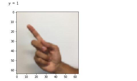
提醒一下，符号数据集是6个符号的集合，它们代表从0到5的数字。

下一个单元格将向您展示数据集中的标记图像示例。您可以随意更改下面的index值并重新运行以查看不同的示例。

# Example of a picture
index = 8
plt.imshow(X_train_orig[index])
print ("y = " + str(np.squeeze(Y_train_orig[:, index])))

运行结果：

在课程2中，您已经为这个数据集构建了一个完全连接的网络。但由于这是一个图像数据集，应用卷积神经网络更自然。

首先，让我们研究一下数据的形状。

在课程2中，我们已经建立过一个神经网络，我想对这个数据集应该不陌生吧~我们再来看一下数据的维度，如果你忘记了独热编码的实现，请看这里

X_train = X_train_orig/255.
X_test = X_test_orig/255.
Y_train = convert_to_one_hot(Y_train_orig, 6).T
Y_test = convert_to_one_hot(Y_test_orig, 6).T
print ("number of training examples = " + str(X_train.shape[0]))
print ("number of test examples = " + str(X_test.shape[0]))
print ("X_train shape: " + str(X_train.shape))
print ("Y_train shape: " + str(Y_train.shape))
print ("X_test shape: " + str(X_test.shape))
print ("Y_test shape: " + str(Y_test.shape))
conv_layers = {}

执行结果：

number of training examples = 1080
number of test examples = 120
X_train shape: (1080, 64, 64, 3)
Y_train shape: (1080, 6)
X_test shape: (120, 64, 64, 3)
Y_test shape: (120, 6)

1.1 - Create placeholders 创建占位符

TensorFlow要求您为运行会话时将输入到模型中的输入数据创建占位符。现在我们要实现创建占位符的函数，因为我们使用的是小批量数据块，输入的样本数量可能不固定，所以我们在数量那里我们要使用None作为可变数量。输入X的维度为**[None,n_H0,n_W0,n_C0]，对应的Y是[None,n_y]**

 1 # GRADED FUNCTION: create_placeholders
 2 
 3 def create_placeholders(n_H0, n_W0, n_C0, n_y):
 4     """
 5     Creates the placeholders for the tensorflow session. 为session创建占位符
 6     
 7     Arguments:
 8     n_H0 -- scalar, height of an input image 实数，输入图像的高度
 9     n_W0 -- scalar, width of an input image 实数，输入图像的宽度
10     n_C0 -- scalar, number of channels of the input 实数，输入的通道数
11     n_y -- scalar, number of classes 实数， 分类数
12         
13     Returns:
14     X -- placeholder for the data input, of shape [None, n_H0, n_W0, n_C0] and dtype "float"
15         输入数据的占位符，维度为[None, n_H0, n_W0, n_C0]，类型为"float"
16     Y -- placeholder for the input labels, of shape [None, n_y] and dtype "float"
17         输入数据的标签的占位符，维度为[None, n_y]，维度为"float"
18     """
19 
20     ### START CODE HERE ### (≈2 lines)
21     X = tf.compat.v1.placeholder(tf.float32, [None, n_H0, n_W0, n_C0])
22     Y = tf.compat.v1.placeholder(tf.float32, [None, n_y])
23     ### END CODE HERE ###
24     
25     return X, Y

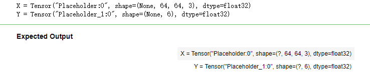
# GRADED FUNCTION: create_placeholders

tf.compat.v1.disable_eager_execution() #这里因为是使用TF2.x的原因，不加会报错

X, Y = create_placeholders(64, 64, 3, 6)
print ("X = " + str(X))
print ("Y = " + str(Y))

执行结果：

tf.placeholder() is not compatible with eager execution的解决方法

1.2 - Initialize parameters 初始化参数

现在我们将使用tf.contrib.layers.xavier_initializer(seed = 0) 来初始化权值/过滤器W1、W2。您不需要担心偏差变量，因为您很快就会看到TensorFlow函数会处理偏差。还要注意，需要注意的是我们只需要初始化为2D卷积函数，全连接层TensorFlow会自动初始化的。

练习:实现initialize_parameters()。下面提供了每组过滤器的尺寸。提醒——初始化参数𝑊形状(1、2、3、4)在Tensorflow,使用:

W = tf.get_variable("W", [1,2,3,4], initializer = ...)

 1 # GRADED FUNCTION: initialize_parameters
 2 
 3 def initialize_parameters():
 4     """
 5     初始化权值矩阵，这里我们把权值矩阵硬编码：
 6     Initializes weight parameters to build a neural network with tensorflow. The shapes are:
 7                         W1 : [4, 4, 3, 8]
 8                         W2 : [2, 2, 8, 16]
 9     Returns:
10     parameters -- a dictionary of tensors containing W1, W2 包含了tensor类型的W1、W2的字典
11     """
12     
13 #     tf.set_random_seed(1)                              # so that your "random" numbers match ours 由于使用tf2.x 所以换成
14     tf.random.set_seed(1)    
15     ### START CODE HERE ### (approx. 2 lines of code)
16     W1 = tf.compat.v1.get_variable('W1', [4, 4, 3, 8], initializer = tf.initializers.GlorotUniform(seed=1))
17     W2 = tf.compat.v1.get_variable('W2', [2, 2, 8, 16], initializer = tf.initializers.GlorotUniform(seed=1))
18     ### END CODE HERE ###
19 
20     parameters = {"W1": W1,
21                   "W2": W2}
22     
23     return parameters

# GRADED FUNCTION: initialize_parameters

# tf.reset_default_graph() 使用的tf2.x 这个不适用
ops.reset_default_graph()
with tf.compat.v1.Session() as sess_test:
    parameters = initialize_parameters()
    init = tf.compat.v1.global_variables_initializer()
    sess_test.run(init)
    print("W1 = " + str(parameters["W1"].eval()[1,1,1]))
    print("W2 = " + str(parameters["W2"].eval()[1,1,1]))

执行结果：

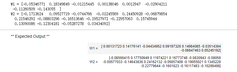
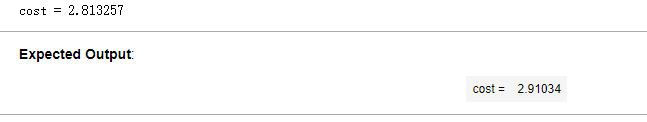
（这里因为是使用tf2.x版本的原因，更改了许多的代码，权重的初始化也换了一个，不知是否是这个原因导致结果和预期不一致）

1.2 - Forward propagation 前向传播

在TensorFlow中，有一些内置函数可以帮你完成卷积步骤。

·tf.nn.conv2d(X,W1, strides = [1,s,s,1], padding = 'SAME'):给定输入 X 和一组过滤器 W1 ，这个函数将会自动使用 W1 来对 X 进行卷积，第三个输入参数是**[1,s,s,1]**是指对于输入（m, n_H_prev, n_W_prev, n_C_prev）而言，每次滑动的步伐。你也可以点这里阅读文档

·tf.nn.max_pool(A, ksize = [1,f,f,1], strides = [1,s,s,1], padding = 'SAME'):给定输入 X ，该函数将会使用大小为（f, f）以及步伐为（s, s）的窗口对其进行滑动取最大值，你也可以看一下文档

·tf.nn.relu(Z1):计算 Z1 的ReLU函数，点这里阅读文档

·tf.contrib.layers.flatten(P):给定一个输入P，此函数将会把每个样本转化成一维的向量，然后返回一个tensor变量，其维度为（batch_size,k）.点这里阅读文档

·tf.contrib.layers.fully_connected(F, num_outputs):给定一个已经一维化了的输入F，此函数将会返回一个由全连接层计算过后的输出。点这里阅读文档

使用tf.contrib.layers.fully_connected(F, num_outputs)的时候，全连接层会自动初始化权值且在你训练模型的时候它也会一直参与，所以当我们初始化参数的时候我们不需要专门去初始化它的权值。

我们实现前向传播的时候，我们需要定义一下我们模型的大概样子：

CONV2D -> RELU -> MAXPOOL -> CONV2D -> RELU -> MAXPOOL -> FLATTEN -> FULLYCONNECTED

我们具体实现的时候，我们需要使用以下的步骤和参数：

Conv2d : 步伐：1，填充方式：“SAME”
ReLU
Max pool : 过滤器大小：8x8，步伐：8x8，填充方式：“SAME”
Conv2d : 步伐：1，填充方式：“SAME”
ReLU
Max pool : 过滤器大小：4x4，步伐：4x4，填充方式：“SAME”
一维化上一层的输出
全连接层（FC）：使用没有非线性激活函数的全连接层。这里不要调用SoftMax，这将导致输出层中有6个神经元，然后再传递到softmax。在TensorFlow中，softmax和cost函数被集中到一个函数中，在计算成本时您将调用不同的函数。

 1 # GRADED FUNCTION: forward_propagation
 2 
 3 def forward_propagation(X, parameters):
 4     """
 5     Implements the forward propagation for the model:  实现前向传播
 6     CONV2D -> RELU -> MAXPOOL -> CONV2D -> RELU -> MAXPOOL -> FLATTEN -> FULLYCONNECTED
 7     
 8     Arguments:
 9     X -- input dataset placeholder, of shape (input size, number of examples) 输入数据的placeholder，维度为(输入节点数量，样本数量)
10     parameters -- python dictionary containing your parameters "W1", "W2"
11                   the shapes are given in initialize_parameters 包含了“W1”和“W2”的python字典。
12 
13     Returns:
14     Z3 -- the output of the last LINEAR unit 最后一个LINEAR节点的输出
15     """
16     
17     # Retrieve the parameters from the dictionary "parameters" 
18     W1 = parameters['W1']
19     W2 = parameters['W2']
20     
21     ### START CODE HERE ###
22     # CONV2D: stride of 1, padding 'SAME'
23     Z1 = tf.nn.conv2d(X, W1, strides=[1, 1, 1, 1], padding = 'SAME')
24     # RELU
25     A1 = tf.nn.relu(Z1)
26     # MAXPOOL: window 8x8, sride 8, padding 'SAME'
27     P1 = tf.nn.max_pool(A1, ksize = [1, 8, 8, 1], strides = [1, 8, 8, 1], padding = 'SAME')
28     # CONV2D: filters W2, stride 1, padding 'SAME'
29     Z2 = tf.nn.conv2d(P1, W2, strides = [1, 1, 1, 1], padding = 'SAME')
30     # RELU
31     A2 = tf.nn.relu(Z2)
32     # MAXPOOL: window 4x4, stride 4, padding 'SAME'
33     P2 = tf.nn.max_pool(A2, ksize = [1, 4, 4, 1], strides = [1, 4, 4, 1], padding = 'SAME')
34     # FLATTEN 一维化，
35     P2 = tf.compat.v1.layers.flatten(P2)
36     
37     # FULLY-CONNECTED without non-linear activation function (not not call softmax).全连接层（FC）：使用没有非线性激活函数的全连接层
38     # 6 neurons in output layer. Hint: one of the arguments should be "activation_fn=None" 
39     Z3 = tf.compat.v1.layers.dense(P2, 6) #这里由于tf2.x删除了contrib，暂时未找到替换的方法，因为跑出的答案不一样
40 #     Z3 = tf.contrib.layers.fully_connected(P,6,activation_fn=None)
41     ### END CODE HERE ###
42 
43     return Z3

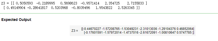
# GRADED FUNCTION: forward_propagation

# tf.reset_default_graph()
ops.reset_default_graph()

with tf.compat.v1.Session() as sess:
    np.random.seed(1)
    X, Y = create_placeholders(64, 64, 3, 6)
    parameters = initialize_parameters()
    Z3 = forward_propagation(X, parameters)
    
    init = tf.compat.v1.global_variables_initializer()
    sess.run(init)
    
    a = sess.run(Z3, {X: np.random.randn(2,64,64,3), Y: np.random.randn(2,6)})
    print("Z3 = " + str(a))
    
    sess.close()

执行结果：

1.3 - Compute cost 计算成本

我们要在这里实现计算成本的函数，下面的两个函数是我们要用到的：

tf.nn.softmax_cross_entropy_with_logits(logits = Z3 , lables = Y)：计算softmax的损失函数。这个函数既计算softmax的激活，也计算其损失，你可以阅读手册
tf.reduce_mean：计算的是平均值，使用它来计算所有样本的损失来得到总成本。你可以阅读手册

现在，我们就来实现计算成本的函数：：

 1 # GRADED FUNCTION: compute_cost 
 2 
 3 def compute_cost(Z3, Y):
 4     """
 5     Computes the cost 计算成本
 6     
 7     Arguments:
 8     Z3 -- output of forward propagation (output of the last LINEAR unit), of shape (6, number of examples)
 9     正向传播最后一个LINEAR节点的输出，维度为（6，样本数）
10     Y -- "true" labels vector placeholder, same shape as Z3
11     标签向量的placeholder，和Z3的维度相同
12     
13     Returns:
14     cost - Tensor of the cost function  代价函数的张量
15     """
16     
17     ### START CODE HERE ### (1 line of code)
18     cost = tf.reduce_mean(tf.nn.softmax_cross_entropy_with_logits(logits = Z3, labels = Y))
19     ### END CODE HERE ###
20     
21     return cost

# GRADED FUNCTION: compute_cost

# tf.reset_default_graph()
ops.reset_default_graph()

with tf.compat.v1.Session() as sess:
    np.random.seed(1)
    X, Y = create_placeholders(64, 64, 3, 6)
    parameters = initialize_parameters()
    Z3 = forward_propagation(X, parameters)
    cost = compute_cost(Z3, Y)
    init = tf.compat.v1.global_variables_initializer()
    sess.run(init)
    a = sess.run(cost, {X: np.random.randn(4,64,64,3), Y: np.random.randn(4,6)})
    print("cost = " + str(a))
    sess.close()

执行结果:

1.4 Model 构建模型

最后，我们已经实现了我们所有的函数，我们现在就可以实现我们的模型了。

我们之前在课程2就实现过random_mini_batches()这个函数，它返回的是一个mini-batches的列表。

在实现这个模型的时候我们要经历以下步骤：

创建占位符
初始化参数
前向传播
计算成本
反向传播
创建优化器

最后，我们将创建一个session来运行模型。

  1 # GRADED FUNCTION: model
  2 
  3 def model(X_train, Y_train, X_test, Y_test, learning_rate = 0.009,
  4           num_epochs = 100, minibatch_size = 64, print_cost = True):
  5     """
  6     Implements a three-layer ConvNet in Tensorflow:     使用TensorFlow实现三层的卷积神经网络
  7     CONV2D -> RELU -> MAXPOOL -> CONV2D -> RELU -> MAXPOOL -> FLATTEN -> FULLYCONNECTED
  8     
  9     Arguments:
 10     X_train -- training set, of shape (None, 64, 64, 3) 训练数据，维度为(None, 64, 64, 3)
 11     Y_train -- test set, of shape (None, n_y = 6) 训练数据对应的标签，维度为(None, n_y = 6)
 12     X_test -- training set, of shape (None, 64, 64, 3) 测试数据，维度为(None, 64, 64, 3)
 13     Y_test -- test set, of shape (None, n_y = 6) 训练数据对应的标签，维度为(None, n_y = 6)
 14     learning_rate -- learning rate of the optimization 学习率
 15     num_epochs -- number of epochs of the optimization loop  遍历整个数据集的次数
 16     minibatch_size -- size of a minibatch 每个小批量数据块的大小
 17     print_cost -- True to print the cost every 100 epochs 是否打印成本值，每遍历100次整个数据集打印一次
 18     
 19     Returns:
 20     train_accuracy -- real number, accuracy on the train set (X_train)  实数，训练集的准确度
 21     test_accuracy -- real number, testing accuracy on the test set (X_test) 实数，测试集的准确度
 22     parameters -- parameters learnt by the model. They can then be used to predict. 学习后的参数，然后可以用作预测
 23     """
 24     
 25     ops.reset_default_graph()                         # to be able to rerun the model without overwriting tf variables 能够重新运行模型而不覆盖tf变量
 26     tf.random.set_seed(1)                             # to keep results consistent (tensorflow seed) 确保你的数据和我一样
 27     seed = 3                                          # to keep results consistent (numpy seed) 指定numpy的随机种子
 28     (m, n_H0, n_W0, n_C0) = X_train.shape             
 29     n_y = Y_train.shape[1]                            
 30     costs = []                                        # To keep track of the cost
 31     
 32     # Create Placeholders of the correct shape 为当前维度创建占位符
 33     ### START CODE HERE ### (1 line)
 34     X, Y = create_placeholders(n_H0, n_W0, n_C0, n_y)
 35     ### END CODE HERE ###
 36 
 37     # Initialize parameters 初始化参数
 38     ### START CODE HERE ### (1 line)
 39     parameters = initialize_parameters()
 40     ### END CODE HERE ###
 41     
 42     # Forward propagation: Build the forward propagation in the tensorflow graph 前向传播：在TensorFlow图中
 43     ### START CODE HERE ### (1 line)
 44     Z3 = forward_propagation(X, parameters)
 45     ### END CODE HERE ###
 46     
 47     # Cost function: Add cost function to tensorflow graph 计算成本
 48     ### START CODE HERE ### (1 line)
 49     cost = compute_cost(Z3, Y)
 50     ### END CODE HERE ###
 51     
 52     # Backpropagation: Define the tensorflow optimizer. Use an AdamOptimizer that minimizes the cost.
 53 #     反向传播，由于框架已经实现了反向传播，我们只需要选择一个优化器就行了
 54     ### START CODE HERE ### (1 line)
 55     optimizer = tf.compat.v1.train.AdamOptimizer(learning_rate = learning_rate).minimize(cost)
 56     ### END CODE HERE ###
 57     
 58     # Initialize all the variables globally 全局初始化所有变量
 59     init = tf.compat.v1.global_variables_initializer()
 60      
 61     # Start the session to compute the tensorflow graph
 62     with tf.compat.v1.Session() as sess:
 63         
 64         # Run the initialization
 65         sess.run(init)
 66         
 67         # Do the training loop 开始遍历数据集
 68         for epoch in range(num_epochs):
 69 
 70             minibatch_cost = 0.
 71             num_minibatches = int(m / minibatch_size) # number of minibatches of size minibatch_size in the train set
 72             seed = seed + 1
 73             minibatches = random_mini_batches(X_train, Y_train, minibatch_size, seed)
 74 
 75             for minibatch in minibatches:
 76 
 77                 # Select a minibatch 选择一个数据块
 78                 (minibatch_X, minibatch_Y) = minibatch
 79                 # IMPORTANT: The line that runs the graph on a minibatch.
 80                 # Run the session to execute the optimizer and the cost, the feedict should contain a minibatch for (X,Y).
 81 #                 最小化这个数据块的成本
 82                 ### START CODE HERE ### (1 line)
 83                 _ , temp_cost = sess.run([optimizer, cost], feed_dict = {X:minibatch_X, Y:minibatch_Y})
 84                 ### END CODE HERE ###
 85 #                 累加数据块的成本值
 86                 minibatch_cost += temp_cost / num_minibatches
 87                 
 88 
 89             # Print the cost every epoch
 90             if print_cost == True and epoch % 5 == 0:
 91                 print ("Cost after epoch %i: %f" % (epoch, minibatch_cost))
 92             if print_cost == True and epoch % 1 == 0:
 93                 costs.append(minibatch_cost)
 94         
 95         
 96         # plot the cost        数据处理完毕，绘制成本曲线
 97         plt.plot(np.squeeze(costs))
 98         plt.ylabel('cost')
 99         plt.xlabel('iterations (per tens)')
100         plt.title("Learning rate =" + str(learning_rate))
101         plt.show()
102 
103          #开始预测数据
104         # Calculate the correct predictions 计算当前的预测情况
105         predict_op = tf.argmax(Z3, 1)
106         correct_prediction = tf.equal(predict_op, tf.argmax(Y, 1))
107         
108         # Calculate accuracy on the test set 计算准确度
109         accuracy = tf.reduce_mean(tf.cast(correct_prediction, "float"))
110         print("corrent_prediction accuracy= " + str(accuracy))
111         
112         train_accuracy = accuracy.eval({X: X_train, Y: Y_train})
113         test_accuracy = accuracy.eval({X: X_test, Y: Y_test})
114         
115         print("Train Accuracy:", train_accuracy)
116         print("Test Accuracy:", test_accuracy)
117                 
118         return train_accuracy, test_accuracy, parameters

# GRADED FUNCTION: model

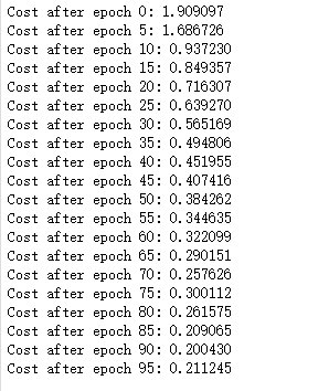
_, _, parameters = model(X_train, Y_train, X_test, Y_test)

执行结果：

恭喜你!您已经完成了任务，并建立了一个在测试集上具有80%准确率的识别手语的模型。如果您愿意，可以进一步使用这个数据集。实际上，您可以通过花费更多时间调优超参数或使用正则化(因为这个模型显然有很高的方差)来提高其准确性。

再一次，我为你的工作竖起大拇指!

posted @ 2020-08-31 11:33 廖海清阅读(3554) 评论(3) 编辑收藏举报

会员力量，点亮园子希望

刷新页面返回顶部

Agiroy_70's Blog

吴恩达深度学习第四课第一周编程作业_Convolutional Neural Networks: Application

Convolutional Neural Networks: Application 卷积神经网络应用

1.0 - TensorFlow model TensorFlow模型

1.1 - Create placeholders 创建占位符

1.2 - Initialize parameters 初始化参数

1.2 - Forward propagation 前向传播

1.3 - Compute cost 计算成本

1.4 Model 构建模型

公告

Agiroy_70's Blog

吴恩达深度学习 第四课第一周编程作业_Convolutional Neural Networks: Application

Convolutional Neural Networks: Application 卷积神经网络应用

1.0 - TensorFlow model TensorFlow模型

1.1 - Create placeholders 创建占位符

1.2 - Initialize parameters 初始化参数

1.2 - Forward propagation 前向传播

1.3 - Compute cost 计算成本

1.4 Model 构建模型

公告

吴恩达深度学习第四课第一周编程作业_Convolutional Neural Networks: Application