吴恩达深度学习第四课第一周编程作业_Convolutional Neural Networks: Step by Step

Convolutional Neural Networks: Step by Step

欢迎来到课程4的第一个作业!在这个任务中，您将在numpy中实现卷积(CONV)和池化层，包括前向传播和(可选的)后向传播。

我们假定你已经熟悉numpy和/或已经完成了该专业的以前的课程。让我们开始吧!

1 - Packages 包

·让我们首先导入在此任务中需要的所有包。

·numpy是使用Python进行科学计算的基本包。
·matplotlib是Python中用于绘制图形的库。
·seed(1)用于保持所有随机函数调用的一致性。它将帮助我们批改你的作业。

import numpy as np
import h5py
import matplotlib.pyplot as plt

%matplotlib inline
plt.rcParams['figure.figsize'] = (5.0, 4.0) # set default size of plots 设置图像的默认大小
plt.rcParams['image.interpolation'] = 'nearest'  # 差值方式
plt.rcParams['image.cmap'] = 'gray' # 灰度空间
#ipython很好用，但是如果在ipython里已经import过的模块修改后需要重新reload就需要这样
#在执行用户代码前，重新装入软件的扩展和模块。
%load_ext autoreload
#autoreload 2：装入所有 %aimport 不包含的模块。
%autoreload 2

np.random.seed(1) #指定随机种子

    是在使用jupyter notebook 或者 jupyter qtconsole的时候，才会经常用到%matplotlib，也就是说那一份代码可能就是别人使用jupyter notebook 或者 jupyter qtconsole进行编辑的。关于jupyter notebook是什么，可以参考这个链接：[Jupyter Notebook介绍、安装及使用教程][1]
    而%matplotlib具体作用是当你调用matplotlib.pyplot的绘图函数plot()进行绘图的时候，或者生成一个figure画布的时候，可以直接在你的python console里面生成图像。

　　（作者：hplllrhp
　　　　链接：https://www.jianshu.com/p/2dda5bb8ce7d
　　　　来源：简书
　　　　著作权归作者所有。商业转载请联系作者获得授权，非商业转载请注明出处。

　　　）

%matplotlib作用

在执行用户代码前，重新装入 软件的扩展和模块。
autoreload 意思是自动重新装入。
它后面可带参数。参数意思你要查你自己的版本帮助文件。一般说：
无参：装入所有模块。
0：不执行 装入命令。
1： 只装入所有 %aimport 要装模块
2：装入所有 %aimport 不包含的模块。

%load_ext autoreload是什么意思

2 - Outline of the Assignment 任务的大纲

您将实现卷积神经网络的构建块!您将实现的每个函数将有详细的说明，将带领您完成所需的步骤:

卷积模块，包含了以下函数：
- 使用0扩充边界
- 卷积窗口
- 前向卷积
- 反向卷积（可选）
池化模块，包含了以下函数：
- 前向池化
- 创建掩码
- 值分配
- 反向池化（可选）

本笔记本将要求您在numpy中从头开始实现这些函数。在下一个笔记本中，您将使用相当于这些函数的TensorFlow来构建以下模型:

注意，对于每个前向函数，都有对应的后向函数。因此，在传播模块的每一步中，您将在缓存中存储一些参数。这些参数用于计算反向传播过程中的梯度。

3 - Convolutional Neural Networks 卷积神经网络

尽管编程框架使卷积易于使用，但它们仍然是深度学习中最难理解的概念之一。卷积层将输入量转换为不同大小的输出量，如下图所示。

在本部分中，您将构建卷积层的每一步。您将首先实现两个辅助函数:一个用于填充零，另一个用于计算卷积函数本身。

3.1 - Zero-Padding 边界填充（填充0）

零填充在图像的边界上增加零:

**Figure 1** : **Zero-Padding**

Image (3 channels, RGB) with a padding of 2.使用pading为2的操作对图像（3通道，RGB）进行填充。

填充的主要好处如下:

卷积了上一层之后的CONV层，没有缩小高度和宽度。这对于建立更深的网络非常重要，否则在更深层时，高度/宽度会缩小。一个重要的例子是“same”卷积，其中高度/宽度在卷积完一层之后会被完全保留。
它可以帮助我们在图像边界保留更多信息。在没有填充的情况下，卷积过程中图像边缘的极少数值会受到过滤器的影响从而导致信息丢失。

我们将实现一个边界填充函数，它会把所有的样本图像 $constant_values = (..,..))$

 1 # GRADED FUNCTION: zero_pad
 2 
 3 def zero_pad(X, pad):
 4     """
 5     Pad with zeros all images of the dataset X. The padding is applied to the height and width of an image, 
 6     as illustrated in Figure 1.
 7     填充应用于图像的高度和宽度，如图1所示。
 8     #constant连续一样的值填充，有constant_values=（x, y）时前面用x填充，后面用y填充。缺省参数是为constant_values=（0,0）
 9     
10     Argument:
11     X -- python numpy array of shape (m, n_H, n_W, n_C) representing a batch of m images 图像数据集，维度为（样本数，图像高度，图像宽度，图像通道数表示一批有m个图像
12     pad -- integer, amount of padding around each image on vertical and horizontal dimensions
13             整数，每个图像在垂直和水平维度上的填充量
14     Returns:
15     X_pad -- padded image of shape (m, n_H + 2*pad, n_W + 2*pad, n_C)
16     扩充后的图像数据集，维度为（样本数，图像高度 + 2*pad，图像宽度 + 2*pad，图像通道数）
17     
18     """
19     
20     ### START CODE HERE ### (≈ 1 line)
21     X_pad = np.pad(X, (
22         (0, 0),    #样本数，不填充
23         (pad, pad),#图像高度,你可以视为上面填充x个，下面填充y个(x,y)
24         (pad, pad),#图像宽度,你可以视为左边填充x个，右边填充y个(x,y)
25         (0, 0)),   #通道数，不填充
26         'constant', constant_values = 0 ) #连续一样的值填充
27     ### END CODE HERE ###
28     
29     return X_pad

# GRADED FUNCTION: zero_pad

np.random.seed(1)
x = np.random.randn(4, 3, 3, 2)
x_pad = zero_pad(x, 2)
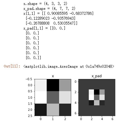
print ("x.shape =", x.shape)
print ("x_pad.shape =", x_pad.shape)
print ("x[1,1] =", x[1,1])
print ("x_pad[1,1] =", x_pad[1,1])

fig, axarr = plt.subplots(1, 2) #一行两列
axarr[0].set_title('x')
axarr[0].imshow(x[0,:,:,0])
axarr[1].set_title('x_pad')
axarr[1].imshow(x_pad[0,:,:,0])

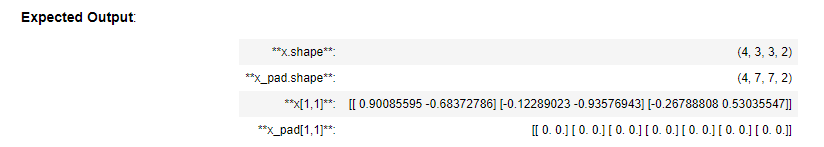
运行结果：

3.2 - Single step of convolution 单步卷积

在计算机视觉应用程序中，左边矩阵中的每个值都对应于一个像素值，我们用一个3x3的过滤器对图像进行卷积，方法是将图像的元素值与原始矩阵相乘，然后将它们相加。在这个练习的第一步中，您将实现卷积的一个步骤，对应于仅对其中一个位置应用一个滤波器来获得一个实值输出。

在本笔记本的后面部分，您将对输入的多个位置应用此函数，以实现完整的卷积操作。

现在我们开始实现conv_single_step()

 1 # GRADED FUNCTION: conv_single_step
 2 
 3 def conv_single_step(a_slice_prev, W, b):
 4     """
 5     Apply one filter defined by parameters W on a single slice (a_slice_prev) of the output activation 
 6     of the previous layer.在前一层的激活输出的一个片段上应用一个由参数W定义的过滤器。这里切片大小和过滤器大小相同
 7     
 8     Arguments:
 9     a_slice_prev -- slice of input data of shape (f, f, n_C_prev) 输入数据的一个片段，维度为（过滤器大小，过滤器大小，上一通道数）
10     W -- Weight parameters contained in a window - matrix of shape (f, f, n_C_prev)
11         权重参数，包含在了一个矩阵中，维度为（过滤器大小，过滤器大小，上一通道数）
12     b -- Bias parameters contained in a window - matrix of shape (1, 1, 1)
13         偏置参数，包含在了一个矩阵中，维度为（1,1,1）
14     
15     Returns:
16     Z -- a scalar value, result of convolving the sliding window (W, b) on a slice x of the input data
17     在输入数据的片X上卷积滑动窗口（w，b）的结果。
18     """
19 
20     ### START CODE HERE ### (≈ 2 lines of code)
21     # Element-wise product between a_slice and W. Add bias.a_slice和w之间的元素积添加偏置。
22     s = np.multiply(a_slice_prev, W) + b
23     # Sum over all entries of the volume s 对s中所有的分量求和
24     Z = np.sum(s)
25     ### END CODE HERE ###
26 
27     return Z

# GRADED FUNCTION: conv_single_step

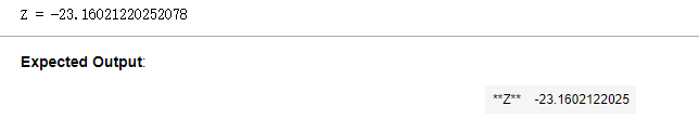
np.random.seed(1)
a_slice_prev = np.random.randn(4, 4, 3)
W = np.random.randn(4, 4, 3)
b = np.random.randn(1, 1, 1)

Z = conv_single_step(a_slice_prev, W, b)
print("Z =", Z)

运行结果：

3.3 - Convolutional Neural Networks - Forward pass 卷积神经网络-前向传播

在前向传递中，您将使用许多过滤器并对输入进行卷积。每个‘卷积’都给你一个2D矩阵输出。然后您将堆叠这些输出，以获得三维体积:

练习:实现下面的函数来对输入激活A_prev进行过滤器的卷积。该函数以A_prev、前一层(对于一批m的输入)输出的激活、F个滤波器/权值(W)和一个偏置向量(b)为输入，其中每个滤波器都有自己的(单个)偏置。最后，您还可以访问包含步幅和填充的超参数字典。

小提示：

1、如果我要在矩阵A_prev（shape = (5,5,3)）的左上角选择一个2x2的矩阵进行切片操作，那么可以这样做：

a_slice_prev = a_prev[0:2,0:2,:]

当您使用将要定义的开始/结束索引在下面定义a_slice_prev时，这将非常有用。

2、如果我想要自定义切片，我们可以这么做：先定义要切片的位置，vert_start、vert_end、 horiz_start、 horiz_end，它们的位置我们看一下下面的图就明白了。

**图 3** : **定义切片的开始、结束位置 (使用 2x2 的过滤器)**

只适用于单通道

提示:卷积的输出形状与输入形状的关系式为:

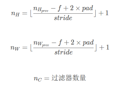
这里我们不会使用矢量化，只是用for循环来实现所有的东西。

 1 # GRADED FUNCTION: conv_forward
 2 
 3 def conv_forward(A_prev, W, b, hparameters):
 4     """
 5     Implements the forward propagation for a convolution function 实现卷积函数的前向传播
 6     
 7     Arguments:
 8     A_prev -- output activations of the previous layer, numpy array of shape (m, n_H_prev, n_W_prev, n_C_prev)
 9          上一层的激活输出矩阵，维度为(m, n_H_prev, n_W_prev, n_C_prev)，（样本数量，上一层图像的高度，上一层图像的宽度，上一层过滤器数量）
10     W -- Weights, numpy array of shape (f, f, n_C_prev, n_C)
11         权重矩阵，维度为(f, f, n_C_prev, n_C)，（过滤器大小，过滤器大小，上一层的过滤器数量，这一层的过滤器数量）
12     b -- Biases, numpy array of shape (1, 1, 1, n_C)
13         偏置矩阵，维度为(1, 1, 1, n_C)，（1,1,1,这一层的过滤器数量）
14     hparameters -- python dictionary containing "stride" and "pad" 包含了"stride"与 "pad"的超参数字典。
15         
16     Returns:
17     Z -- conv output, numpy array of shape (m, n_H, n_W, n_C)卷积输出，维度为(m, n_H, n_W, n_C)，（样本数，图像的高度，图像的宽度，过滤器数量）
18     cache -- cache of values needed for the conv_backward() function 缓存了一些反向传播函数conv_backward()需要的一些数据
19     """
20     
21     ### START CODE HERE ###
22     # Retrieve dimensions from A_prev's shape (≈1 line)  获取来自上一层数据的基本信息
23     (m, n_H_prev, n_W_prev, n_C_prev) = A_prev.shape
24     
25     # Retrieve dimensions from W's shape (≈1 line) 获取权重矩阵的基本信息
26     (f, f, n_C_prev, n_C) = W.shape
27     
28     # Retrieve information from "hparameters" (≈2 lines)获取超参数hparameters的值
29     stride = hparameters['stride']
30     pad = hparameters['pad']
31     
32     # Compute the dimensions of the CONV output volume using the formula given above. Hint: use int() to floor. (≈2 lines)
33 #     计算卷积后的图像的宽度高度，参考上面的公式，使用int()来进行板除
34     n_H = int((n_H_prev + 2 * pad - f) / stride) + 1
35     n_W = int((n_W_prev + 2 * pad - f) / stride) + 1
36     
37     # Initialize the output volume Z with zeros. (≈1 line) 使用0来初始化卷积输出Z
38     Z = np.zeros((m, n_H, n_W, n_C))
39     
40     # Create A_prev_pad by padding A_prev 通过A_prev创建填充过了的A_prev_pad
41     A_prev_pad = zero_pad(A_prev, pad)
42     
43     for i in range(m):                               # loop over the batch of training examples 遍历样本
44         a_prev_pad = A_prev_pad[i]                               # Select ith training example's padded activation 选择第i个样本的扩充后的激活矩阵
45         for h in range(n_H):                           # loop over vertical axis of the output volume 在输出的垂直轴上循环
46             for w in range(n_W):                       # loop over horizontal axis of the output volume 在输出的水平轴上循环
47                 for c in range(n_C):                   # loop over channels (= #filters) of the output volume 循环遍历输出的通道
48                     
49                     # Find the corners of the current "slice" (≈4 lines) 定位当前的切片位置
50                     vert_start = h * stride    #竖向，开始的位置
51                     vert_end = vert_start + f  #竖向，结束的位置
52                     horiz_start = w * stride   #横向，开始的位置
53                     horiz_end = horiz_start + f  #横向，结束的位置
54                     
55                     #切片位置定位好了我们就把它取出来,需要注意的是我们是“穿透”取出来的，
56                     #自行脑补一下吸管插入一层层的橡皮泥就明白了
57                     
58                     # Use the corners to define the (3D) slice of a_prev_pad (See Hint above the cell). (≈1 line)
59                     a_slice_prev = a_prev_pad[vert_start:vert_end, horiz_start:horiz_end, : ]
60                     
61                      #执行单步卷积
62                     # Convolve the (3D) slice with the correct filter W and bias b, to get back one output neuron. (≈1 line)
63                     Z[i, h, w, c] = conv_single_step(a_slice_prev, W[:, :, :, c ], b[0, 0, 0, c])
64                                         
65     ### END CODE HERE ###
66     
67     # Making sure your output shape is correct 数据处理完毕，验证数据格式是否正确
68     assert(Z.shape == (m, n_H, n_W, n_C))
69     
70     # Save information in "cache" for the backprop 存储一些缓存值，以便于反向传播使用
71     cache = (A_prev, W, b, hparameters)
72     
73     return Z, cache

# GRADED FUNCTION: conv_forward

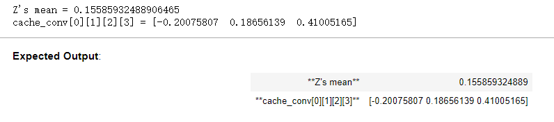
np.random.seed(1)
A_prev = np.random.randn(10,4,4,3)
W = np.random.randn(2,2,3,8)
b = np.random.randn(1,1,1,8)
hparameters = {"pad" : 2,
               "stride": 1}

Z, cache_conv = conv_forward(A_prev, W, b, hparameters)
print("Z's mean =", np.mean(Z))
print("cache_conv[0][1][2][3] =", cache_conv[0][1][2][3])

运行结果：

最后，卷积层应该包含一个激活函数，我们可以加一行代码来计算：

#获取输出
Z[i, h, w, c] = ...
#计算激活
A[i, h, w, c] = activation(Z[i, h, w, c])

不过，在这里我们不需要这么做。

4 - Pooling layer 池化层

池化层会减少输入的宽度和高度，这样它会较少计算量的同时也使特征检测器对其在输入中的位置更加稳定。下面介绍两种类型的池化层：

·最大值池化层：在输入矩阵中滑动一个大小为 f x f 的窗口，选取窗口里的值中的最大值，然后作为输出的一部分。

均值池化层：在输入矩阵中滑动一个大小为 f x f 的窗口，计算窗口里的值中的平均值，然后这个均值作为输出的一部分。

池化层没有用于进行反向传播的参数，但是它们有像窗口的大小为

4.1 - Forward Pooling 池化层的前向传播

现在，您将在同一个函数中实现MAX-POOL和AVG-POOL。

练习:实现池化层的转发。请遵循下面评论中的提示。

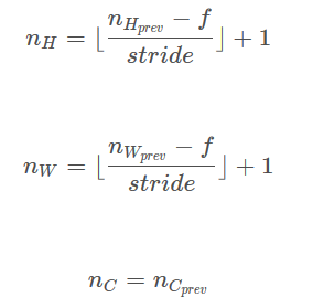
提示:由于没有填充，将池的输出形状绑定到输入形状的公式为:

 1 # GRADED FUNCTION: pool_forward
 2 
 3 def pool_forward(A_prev, hparameters, mode = "max"):
 4     """
 5     Implements the forward pass of the pooling layer 实现池化层的前向传播
 6     
 7     Arguments:
 8     A_prev -- Input data, numpy array of shape (m, n_H_prev, n_W_prev, n_C_prev) 输入数据，维度为(m, n_H_prev, n_W_prev, n_C_prev)
 9     hparameters -- python dictionary containing "f" and "stride" 包含了 "f" 和 "stride"的超参数字典
10     mode -- the pooling mode you would like to use, defined as a string ("max" or "average") 模式选择【"max" | "average"】
11      
12     Returns:
13     A -- output of the pool layer, a numpy array of shape (m, n_H, n_W, n_C) 池化层的输出，维度为 (m, n_H, n_W, n_C)
14     cache -- cache used in the backward pass of the pooling layer, contains the input and hparameters 存储了一些反向传播需要用到的值，包含了输入和超参数的字典。 
15     """
16     
17     # Retrieve dimensions from the input shape 获取输入数据的基本信息
18     (m, n_H_prev, n_W_prev, n_C_prev) = A_prev.shape
19     
20     # Retrieve hyperparameters from "hparameters" 获取超参数的信息
21     f = hparameters["f"]
22     stride = hparameters["stride"]
23     
24     # Define the dimensions of the output 计算输出维度
25     n_H = int(1 + (n_H_prev - f) / stride)
26     n_W = int(1 + (n_W_prev - f) / stride)
27     n_C = n_C_prev
28     
29     # Initialize output matrix A 初始化输出矩阵
30     A = np.zeros((m, n_H, n_W, n_C))              
31     
32     ### START CODE HERE ###
33     for i in range(m):                         # loop over the training examples 遍历样本
34         for h in range(n_H):                     # loop on the vertical axis of the output volume 在输出的垂直轴上循环
35             for w in range(n_W):                 # loop on the horizontal axis of the output volume 在输出的水平轴上循环
36                 for c in range (n_C):            # loop over the channels of the output volume 循环遍历输出的通道
37                     
38                     
39                     # Find the corners of the current "slice" (≈4 lines) 定位当前的切片位置
40                     vert_start = h * stride
41                     vert_end = vert_start + f
42                     horiz_start = w * stride
43                     horiz_end = horiz_start + f
44                     
45                     # Use the corners to define the current slice on the ith training example of A_prev, channel c. (≈1 line)
46                     a_prev_slice = A_prev[i, vert_start:vert_end, horiz_start:horiz_end, c]
47                     
48                     # Compute the pooling operation on the slice. Use an if statment to differentiate the modes. Use np.max/np.mean.
49                     
50                     if mode == "max":
51                         A[i, h, w, c] = np.max(a_prev_slice)
52                     elif mode == "average":
53                         A[i, h, w, c] = np.mean(a_prev_slice)
54     
55     ### END CODE HERE ###
56     
57     # Store the input and hparameters in "cache" for pool_backward() 开始存储用于反向传播的值
58     cache = (A_prev, hparameters)
59     
60     # Making sure your output shape is correct 池化完毕，校验数据格式
61     assert(A.shape == (m, n_H, n_W, n_C))
62     
63     return A, cache

# GRADED FUNCTION: pool_forward

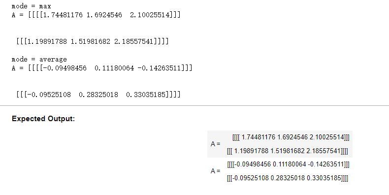
np.random.seed(1)
A_prev = np.random.randn(2, 4, 4, 3)
hparameters = {"stride" : 1, "f": 4}

A, cache = pool_forward(A_prev, hparameters)
print("mode = max")
print("A =", A)
print()
A, cache = pool_forward(A_prev, hparameters, mode = "average")
print("mode = average")
print("A =", A)

运行结果：

恭喜你!现在，您已经实现了卷积网络所有层的转发传递。

本笔记本的剩余部分是可选的，不会评分。

5 - Backpropagation in convolutional neural networks (OPTIONAL / UNGRADED) 卷积神经网络中的反向传播(可选/未分级)

$在现代的深度学习框架中，你只需要实现前向传递，而框架会处理后向传递，所以大多数深度学习工程师不需要费心处理后向传递的细节。卷积网络的反向传递是复杂的。但是，如果您愿意，您可以查看这个笔记本的可选部分，以了解卷积网络中的backprop是什么样子。在前面的课程中，您实现了一个简单的(完全连接的)神经网络，您使用了反向传播来计算与更新参数的代价相关的导数。类似地，在卷积神经网络中，你可以计算关于代价的导数来更新参数。这些反向传播的公式并不简单，我们在课堂上没有推导过它们，但我们在下面简要介绍了它们。$

5.1 - Convolutional layer backward pass 卷积层的反向传播

我们来看一下如何实现卷积层的反向传播

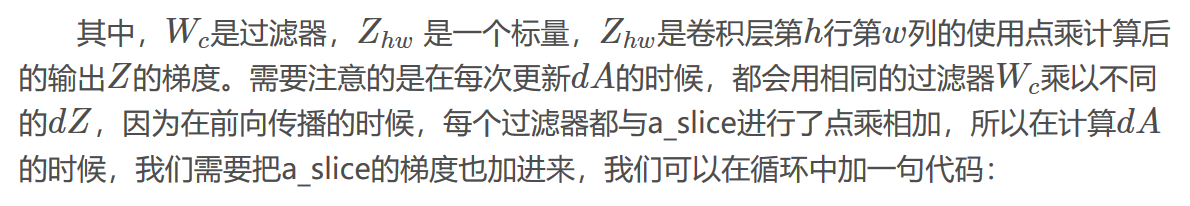
5.1.1 - Computing dA: 计算dA

这是公式计算𝑑𝐴对某个过滤器的成本𝑊𝑐和给定的训练示例:

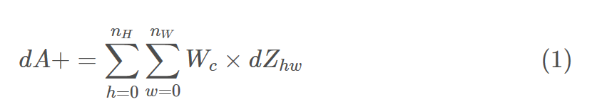
da_prev_pad[vert_start:vert_end, horiz_start:horiz_end, :] += W[:,:,:,c] * dZ[i, h, w, c]

5.1.2 - Computing dW:计算dW

这是计算的公式（是一个过滤器的梯度）：

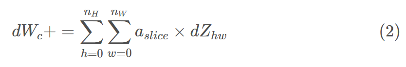
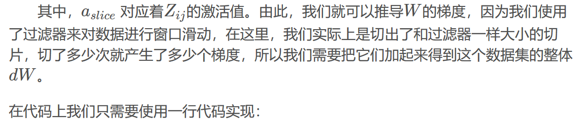
在代码上我们只需要使用一行代码实现：

dW[:,:,:,c] += a_slice * dZ[i, h, w, c]

5.1.3 - Computing db:

这是公式计算𝑑𝑏对某个过滤器的成本𝑊𝑐:

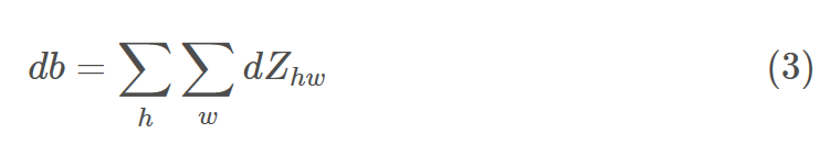
你以前见过的基本神经网络,数据库由加法计算𝑑𝑍。在这种情况下，您只是将conv输出(Z)相对于代价的所有梯度相加。

在代码中，在合适的for循环中，这个公式可以转化为:

db[:,:,:,c] += dZ[i, h, w, c]

练习:实现下面的conv_backward函数。您应该对所有训练示例、过滤器、高度和宽度进行求和。然后使用上面的公式1、2和3计算导数。

 1 def conv_backward(dZ, cache):
 2     """
 3     Implement the backward propagation for a convolution function 实现卷积层的反向传播
 4     
 5     Arguments:
 6     dZ -- gradient of the cost with respect to the output of the conv layer (Z), numpy array of shape (m, n_H, n_W, n_C)
 7     dZ - 卷积层的输出Z的 梯度，维度为(m, n_H, n_W, n_C)
 8     cache -- cache of values needed for the conv_backward(), output of conv_forward()
 9     cache - 反向传播所需要的参数，conv_forward()的输出之一
10     
11     Returns:
12     dA_prev -- gradient of the cost with respect to the input of the conv layer (A_prev),
13                numpy array of shape (m, n_H_prev, n_W_prev, n_C_prev)
14                dA_prev - 卷积层的输入（A_prev）的梯度值，维度为(m, n_H_prev, n_W_prev, n_C_prev)
15     dW -- gradient of the cost with respect to the weights of the conv layer (W)
16           numpy array of shape (f, f, n_C_prev, n_C)
17           卷积层的权值的梯度，维度为(f,f,n_C_prev,n_C)
18     db -- gradient of the cost with respect to the biases of the conv layer (b)
19           numpy array of shape (1, 1, 1, n_C)
20           卷积层的偏置的梯度，维度为（1,1,1,n_C）
21     """
22     
23     ### START CODE HERE ###
24     # Retrieve information from "cache" 获取cache的值
25     (A_prev, W, b, hparameters) = cache
26     
27     # Retrieve dimensions from A_prev's shape 获取A_prev的基本信息
28     (m, n_H_prev, n_W_prev, n_C_prev) = A_prev.shape
29     
30     # Retrieve dimensions from W's shape 获取权值的基本信息
31     (f, f, n_C_prev, n_C) = W.shape
32     
33     # Retrieve information from "hparameters"获取hparaeters的值
34     stride = hparameters['stride']
35     pad = hparameters['pad']
36     
37     # Retrieve dimensions from dZ's shape 获取dZ的基本信息
38     (m, n_H, n_W, n_C) = dZ.shape
39     
40     # Initialize dA_prev, dW, db with the correct shapes 初始化各个梯度的结构
41     dA_prev = np.zeros((m, n_H_prev, n_W_prev, n_C_prev))                           
42     dW = np.zeros((f, f, n_C_prev, n_C))
43     db = np.zeros((1, 1, 1, n_C))
44 
45     # Pad A_prev and dA_prev  前向传播中我们使用了pad，反向传播也需要使用，这是为了保证数据结构一致
46     A_prev_pad = zero_pad(A_prev, pad)
47     dA_prev_pad = zero_pad(dA_prev, pad)
48     
49     for i in range(m):                       # loop over the training examples
50         
51         #选择第i个扩充了的数据的样本,降了一维。
52         # select ith training example from A_prev_pad and dA_prev_pad
53         a_prev_pad = A_prev_pad[i]
54         da_prev_pad = dA_prev_pad[i]
55         
56         for h in range(n_H):                   # loop over vertical axis of the output volume
57             for w in range(n_W):               # loop over horizontal axis of the output volume
58                 for c in range(n_C):           # loop over the channels of the output volume
59                     
60                     # Find the corners of the current "slice" 定义切片位置
61                     vert_start = h * stride
62                     vert_end = vert_start + f
63                     horiz_start = w * stride
64                     horiz_end = horiz_start + f
65                     
66                     # Use the corners to define the slice from a_prev_pad 定位完毕，开始切片
67                     a_slice = a_prev_pad[vert_start:vert_end, horiz_start:horiz_end, :]
68 
69                     # Update gradients for the window and the filter's parameters using the code formulas given above
70                     #切片完毕，使用上面的公式计算梯度
71                     da_prev_pad[vert_start:vert_end, horiz_start:horiz_end, :] += W[:, :, :, c] * dZ[i, h, w, c]
72                     dW[:,:,:,c] += a_slice * dZ[i, h, w, c]
73                     db[:,:,:,c] += dZ[i, h, w, c]
74                     
75         # Set the ith training example's dA_prev to the unpaded da_prev_pad (Hint: use X[pad:-pad, pad:-pad, :])
76         #设置第i个样本最终的dA_prev,即把非填充的数据取出来。
77         dA_prev[i, :, :, :] = da_prev_pad[pad:-pad, pad:-pad, :]
78     ### END CODE HERE ###
79     
80     # Making sure your output shape is correct 数据处理完毕，验证数据格式是否正确
81     assert(dA_prev.shape == (m, n_H_prev, n_W_prev, n_C_prev))
82     
83     return dA_prev, dW, db

def conv_backward(dZ, cache):

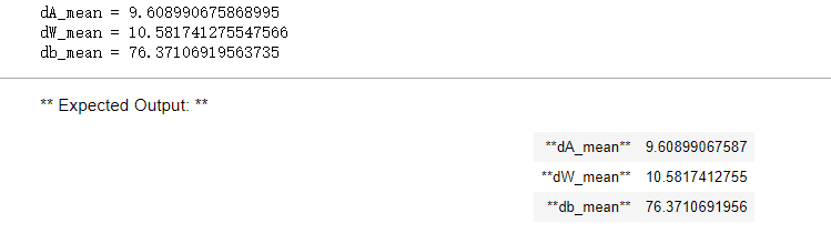
np.random.seed(1)
dA, dW, db = conv_backward(Z, cache_conv)
print("dA_mean =", np.mean(dA))
print("dW_mean =", np.mean(dW))
print("db_mean =", np.mean(db))

运行结果：

5.2 Pooling layer - backward pass 池化层-反向传播

接下来，让我们实现池化层的向后传递，从最大池层开始。即使池化层没有backprop要更新的参数，您仍然需要通过池化层反向传播梯度，以便计算在池化层之前出现的层的梯度。

5.2.1 Max pooling - backward pass 最大值池化层-反向传播

在开始池化层的反向传播之前，我们需要创建一个create_mask_from_window()的函数，我们来看一下它是干什么的：

正如你所看到的，这个函数创建了一个掩码矩阵，以保存最大值的位置，当为1的时候表示最大值的位置，其他的为0，这个是最大值池化层，均值池化层的向后传播也和这个差不多，但是使用的是不同的掩码。

练习:实现create_mask_from_window()。这个函数将有助于向后池化。提示:

　　np.max()可能有帮助。它计算数组的最大值。

　　如果你有一个矩阵X和一个标量X: a = (X == x)会返回一个和X大小相同的矩阵a：

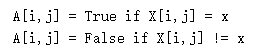
在这里，您不需要考虑一个矩阵中有几个极大值的情况。

 1 def create_mask_from_window(x):
 2     """
 3     Creates a mask from an input matrix x, to identify the max entry of x.
 4     从输入矩阵中创建掩码，以保存最大值的矩阵的位置。
 5     
 6     Arguments:
 7     x -- Array of shape (f, f) 一个维度为(f,f)的矩阵
 8     
 9     Returns:
10     mask -- Array of the same shape as window, contains a True at the position corresponding to the max entry of x.
11     包含x的最大值的位置的矩阵
12     """
13     
14     ### START CODE HERE ### (≈1 line)
15     mask = x == np.max(x) #这里的最大值是其他都为0吗？
16     ### END CODE HERE ###
17     
18     return mask

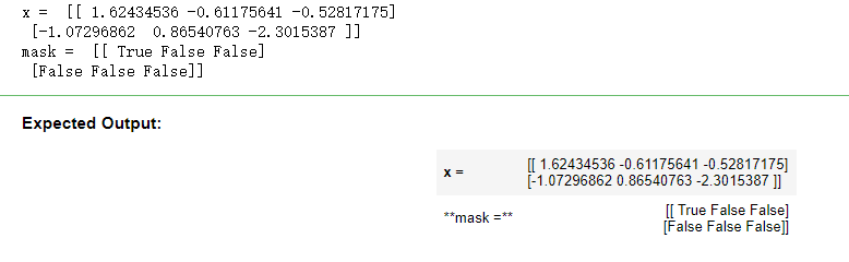
np.random.seed(1)
x = np.random.randn(2,3)
mask = create_mask_from_window(x)
print('x = ', x)
print("mask = ", mask)

运行结果：

为什么我们要跟踪最大值的位置?这是因为输入值最终影响了输出，因此也影响了成本。Backprop是计算相对于代价的梯度，所以任何影响最终代价的东西都应该有一个非零的梯度。因此，backprop会将梯度“传播”回这个影响成本的特定输入值。

5.2.2 - Average pooling - backward pass 均值池化-反向传播

在max pooling中，对于每个输入窗口，对输出的所有“影响”都来自一个输入值——max。在平均池中，输入窗口的每个元素对输出的影响是相等的。因此，要实现backprop，现在需要实现一个辅助函数来反映这一点。

例如，如果我们使用一个2x2的过滤器在前向传递中进行平均池化，那么你将用于后向传递的掩码是这样的:

这意味着每个位置𝑑𝑍矩阵同样有助于输出因为在向前传播,我们平均了。

练习:实现下面的函数，通过维度形状矩阵平均分配值dz。

def distribute_value(dz, shape):
    """
    Distributes the input value in the matrix of dimension shape
    给定一个值，为按矩阵大小平均分配到每一个矩阵位置中。
    
    Arguments: 
    dz -- input scalar 输入的实数
    shape -- the shape (n_H, n_W) of the output matrix for which we want to distribute the value of dz
    元组，两个值，分别为n_H , n_W
    
    Returns:
    a -- Array of size (n_H, n_W) for which we distributed the value of dz 已经分配好了值的矩阵，里面的值全部一样。
    """
    
    ### START CODE HERE ###获取矩阵的大小
    # Retrieve dimensions from shape (≈1 line)
    (n_H, n_W) = shape
    
    # Compute the value to distribute on the matrix (≈1 line) 计算平均值
    average = dz / (n_H * n_W)
    
    # Create a matrix where every entry is the "average" value (≈1 line) 填充入矩阵
    a = np.ones(shape) * average #创建一个都是1的矩阵，在乘上均值
    ### END CODE HERE ###
    
    return a

a = distribute_value(2, (2,2))
print('distributed value =', a)

运行结果：

5.2.3 Putting it together: Pooling backward 池化层的反向传播

现在您已经拥有了在池化层上计算向后传播所需的一切。

练习:在两种模式下(“max”和“average”)实现pool_backward函数。您将再次使用4个for循环(遍历训练示例、高度、宽度和通道)。您应该使用if/elif语句来查看模式是等于“max”还是“average”。如果它等于'average'，那么应该使用上面实现的distribute_value()函数创建一个与a_slice形状相同的矩阵。否则，模式等于'max'，您将使用create_mask_from_window()创建一个掩码，并将其乘以相应的dZ值。

 1 def pool_backward(dA, cache, mode = "max"):
 2     """
 3     Implements the backward pass of the pooling layer  实现池化层的反向传播
 4     
 5     Arguments:
 6     dA -- gradient of cost with respect to the output of the pooling layer, same shape as A
 7         dA - 池化层的输出的梯度，和池化层的输出的维度一样
 8     cache -- cache output from the forward pass of the pooling layer, contains the layer's input and hparameters 
 9         cache - 池化层前向传播时所存储的参数。
10     mode -- the pooling mode you would like to use, defined as a string ("max" or "average")
11         mode - 模式选择，【"max" | "average"】
12         
13     Returns:
14     dA_prev -- gradient of cost with respect to the input of the pooling layer, same shape as A_prev
15         dA_prev - 池化层的输入的梯度，和A_prev的维度相同
16         
17     """
18     
19     ### START CODE HERE ###
20     
21     # Retrieve information from cache (≈1 line) 获取cache中的值
22     (A_prev, hparameters) = cache
23     
24     # Retrieve hyperparameters from "hparameters" (≈2 lines) 获取hparaeters的值
25     stride = hparameters['stride']
26     f = hparameters['f']
27     
28     # Retrieve dimensions from A_prev's shape and dA's shape (≈2 lines) 获取A_prev和dA的基本信息
29     m, n_H_prev, n_W_prev, n_C_prev = A_prev.shape
30     m, n_H, n_W, n_C = dA.shape
31     
32     # Initialize dA_prev with zeros (≈1 line)初始化输出的结构
33     dA_prev = np.zeros_like(A_prev)
34     
35     for i in range(m):                       # loop over the training examples
36         
37         # select training example from A_prev (≈1 line)
38         a_prev = A_prev[i]
39         
40         for h in range(n_H):                   # loop on the vertical axis
41             for w in range(n_W):               # loop on the horizontal axis
42                 for c in range(n_C):           # loop over the channels (depth)
43                     
44                     # Find the corners of the current "slice" (≈4 lines) 定义切片的位置
45                     vert_start = h * stride
46                     vert_end = vert_start + f
47                     horiz_start = w * stride
48                     horiz_end = horiz_start + f
49                     
50                     # Compute the backward propagation in both modes. #选择反向传播的计算方式
51                     if mode == "max":
52                         
53                         # Use the corners and "c" to define the current slice from a_prev (≈1 line)
54                         a_prev_slice = a_prev[vert_start:vert_end, horiz_start:horiz_end, c]
55                         # Create the mask from a_prev_slice (≈1 line)
56                         mask = create_mask_from_window(a_prev_slice) #前面写过的函数
57                         # Set dA_prev to be dA_prev + (the mask multiplied by the correct entry of dA) (≈1 line) 计算dA_prev
58                         dA_prev[i, vert_start: vert_end, horiz_start: horiz_end, c] += np.multiply(mask, dA[i, h, w, c])
59                         
60                     elif mode == "average":
61                         
62                         # Get the value a from dA (≈1 line) 获取dA的值
63                         da = dA[i, h, w, c]
64                         # Define the shape of the filter as fxf (≈1 line) 定义过滤器大小
65                         shape = (f, f)
66                         # Distribute it to get the correct slice of dA_prev. i.e. Add the distributed value of da. (≈1 line)
67                         dA_prev[i, vert_start: vert_end, horiz_start: horiz_end, c] += distribute_value(da, shape)
68                         
69     ### END CODE ###
70     
71     # Making sure your output shape is correct数据处理完毕，开始验证格式
72     assert(dA_prev.shape == A_prev.shape)
73     
74     return dA_prev

def pool_backward(dA, cache, mode = "max"):

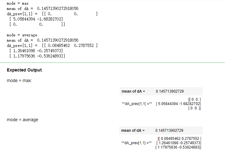
np.random.seed(1)
A_prev = np.random.randn(5, 5, 3, 2)
hparameters = {"stride" : 1, "f": 2}
A, cache = pool_forward(A_prev, hparameters)
dA = np.random.randn(5, 4, 2, 2)

dA_prev = pool_backward(dA, cache, mode = "max")
print("mode = max")
print('mean of dA = ', np.mean(dA))
print('dA_prev[1,1] = ', dA_prev[1,1])  
print()
dA_prev = pool_backward(dA, cache, mode = "average")
print("mode = average")
print('mean of dA = ', np.mean(dA))
print('dA_prev[1,1] = ', dA_prev[1,1])

运行结果：

Congratulations !

恭喜你完成了这项任务。现在您已经了解了卷积神经网络是如何工作的。您已经实现了神经网络的所有构建模块。在下一个作业中，您将使用TensorFlow实现一个卷积网。

posted @ 2020-08-27 21:59 廖海清阅读(1020) 评论(0) 编辑收藏举报

会员力量，点亮园子希望

刷新页面返回顶部

Agiroy_70's Blog

吴恩达深度学习第四课第一周编程作业_Convolutional Neural Networks: Step by Step

Convolutional Neural Networks: Step by Step

1 - Packages 包

2 - Outline of the Assignment 任务的大纲

3 - Convolutional Neural Networks 卷积神经网络

3.1 - Zero-Padding 边界填充（填充0）

3.2 - Single step of convolution 单步卷积

3.3 - Convolutional Neural Networks - Forward pass 卷积神经网络-前向传播

4 - Pooling layer 池化层

4.1 - Forward Pooling 池化层的前向传播

5 - Backpropagation in convolutional neural networks (OPTIONAL / UNGRADED) 卷积神经网络中的反向传播(可选/未分级)

5.1 - Convolutional layer backward pass 卷积层的反向传播

5.1.1 - Computing dA: 计算dA

5.1.2 - Computing dW:计算dW

5.1.3 - Computing db:

5.2 Pooling layer - backward pass 池化层-反向传播

5.2.1 Max pooling - backward pass 最大值池化层-反向传播

5.2.2 - Average pooling - backward pass 均值池化-反向传播

5.2.3 Putting it together: Pooling backward 池化层的反向传播

公告

Agiroy_70's Blog

吴恩达深度学习 第四课第一周编程作业_Convolutional Neural Networks: Step by Step

Convolutional Neural Networks: Step by Step

1 - Packages 包

2 - Outline of the Assignment 任务的大纲

3 - Convolutional Neural Networks 卷积神经网络

3.1 - Zero-Padding 边界填充（填充0）

3.2 - Single step of convolution 单步卷积

3.3 - Convolutional Neural Networks - Forward pass 卷积神经网络-前向传播

4 - Pooling layer 池化层

4.1 - Forward Pooling 池化层的前向传播

5 - Backpropagation in convolutional neural networks (OPTIONAL / UNGRADED) 卷积神经网络中的反向传播(可选/未分级)

5.1 - Convolutional layer backward pass 卷积层的反向传播

5.1.1 - Computing dA: 计算dA

5.1.2 - Computing dW:计算dW

5.1.3 - Computing db:

5.2 Pooling layer - backward pass 池化层-反向传播

5.2.1 Max pooling - backward pass 最大值池化层-反向传播

5.2.2 - Average pooling - backward pass 均值池化-反向传播

5.2.3 Putting it together: Pooling backward 池化层的反向传播

公告

吴恩达深度学习第四课第一周编程作业_Convolutional Neural Networks: Step by Step