吴恩达深度学习第二课第三周编程作业_TensorFlow Tutorial TensorFlow教程

TensorFlow Tutorial TensorFlow教程

欢迎来到本周的编程作业。到目前为止，您一直使用numpy来构建神经网络。现在我们将引导你通过一个深度学习框架，它将允许你更容易地建立神经网络。像TensorFlow, PaddlePaddle, Torch, Caffe, Keras等机器学习框架可以显著加快你机器学习的发展。所有这些框架都有大量文档，您可以随意阅读。在这个作业中，你将学习在TensorFlow中完成以下操作:

初始化变量
开始你自己的会话
训练算法
实现一个神经网络

编程框架不仅可以缩短您的编码时间，有时还可以执行优化来加速您的代码。

1 - Exploring the Tensorflow Library 探索Tensorflow库

首先，您将导入库:

 1 import math
 2 import numpy as np
 3 import h5py
 4 import matplotlib.pyplot as plt
 5 import tensorflow as tf
 6 from tensorflow.python.framework import ops
 7 from tf_utils import load_dataset, random_mini_batches, convert_to_one_hot, predict
 8 
 9 %matplotlib inline
10 np.random.seed(1)

现在您已经导入了库，我们将带您浏览它的不同应用程序。你将从一个例子开始，我们计算一个训练例子的损失。

原代码为：

y_hat = tf.constant(36, name='y_hat')            # Define y_hat constant. Set to 36.
y = tf.constant(39, name='y')                    # Define y. Set to 39

loss = tf.Variable((y - y_hat)**2, name='loss')  # Create a variable for the loss

init = tf.global_variables_initializer()         # When init is run later (session.run(init)),
                                                 # the loss variable will be initialized and ready to be computed
with tf.Session() as session:                    # Create a session and print the output
    session.run(init)                            # Initializes the variables
    print(session.run(loss))                     # Prints the loss

根据网上参考，适应tf2.0版本修改的：

import tensorflow as tf
tf.compat.v1.disable_eager_execution()           #保证session.run()能够正常运行
y_hat = tf.constant(36, name='y_hat')            # Define y_hat constant. Set to 36.
y = tf.constant(39, name='y')                    # Define y. Set to 39
 
loss = tf.Variable((y - y_hat)**2, name='loss')  # Create a variable for the loss
init = tf.compat.v1.global_variables_initializer()         # When init is run later (session.run(init)),
                                    # the loss variable will be initialized and ready to be computed
with tf.compat.v1.Session () as session:                    # Create a session and print the output
    session.run(init)                            # Initializes the variables
    print(session.run(loss))

运行结果：

在TensorFlow中编写和运行程序有以下步骤:

1、创建Tensorflow变量（此时，尚未直接计算）
2、实现Tensorflow变量之间的操作定义。
3、初始化Tensorflow变量
4、创建一个会话，也就是session。
5、运行会话。这将运行您上面所写的操作。

因此，当我们为损失创建一个变量时，我们只是将损失定义为其他数量的函数，但没有计算它的值。要对它求值，我们必须运行init=tf.global_variables_initializer()。这样就初始化了loss变量，并且在最后一行中，我们终于能够计算loss的值并打印它的值。

现在让我们看一个简单的例子。运行下面的单元格:
　　（链接：https://blog.csdn.net/weixin_47440593/article/details/107721334

　　参考的博客为https://blog.csdn.net/u013733326/article/details/79971488

　　原博客中作者用的是tf1.x版本的，本文用的是tf2.x版本，这里挂一下网友整理的两个版本更新的对比https://docs.qq.com/sheet/DZkR6cUZpdFJ2bUxS?tab=BB08J2

　　tensorflow2.0用1.0的代码

　　）

a = tf.constant(2)
b = tf.constant(10)
c = tf.multiply(a,b)
print(c)

运行结果：

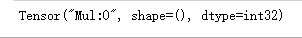
正如所料，您不会看到20!你得到一个变量，说结果是一个没有形状属性的张量（没有维度），类型是“int32”。你所做的一切都被放到了“计算图(computation graph)”中，但是你还没有运行这个计算。为了实际地将两个数字相乘，您必须创建一个会话并运行它。

sess = tf.compat.v1.Session()
print(sess.run(c))

运行结果：

太棒了!总之，请记住初始化变量、创建会话并在会话内运行操作。

接下来，您还需要了解占位符。占位符是只能在以后指定其值的对象。要为占位符指定值，可以使用“feed字典”(feed_dict变量)传入值。下面，我们为x创建了一个占位符。这允许我们在稍后运行会话时传入一个数字。

# Change the value of x in the feed_dict

x = tf.compat.v1.placeholder(tf.int64, name = 'x')
print(sess.run(2 * x, feed_dict = {x: 3}))
sess.close()

运行结果：

placeholder means '占位符'

tf.placeholder函数说明

当你第一次定义x时，你不需要为它指定一个值。占位符只是一个变量，您将在稍后运行会话时将数据分配给它。我们说，在运行会话时向这些占位符提供数据。

当您指定一个计算所需的操作时，您正在告诉TensorFlow如何构造一个计算图。计算图中可以有一些占位符，它们的值将稍后指定。最后，当您运行会话时，您告诉TensorFlow执行计算图。

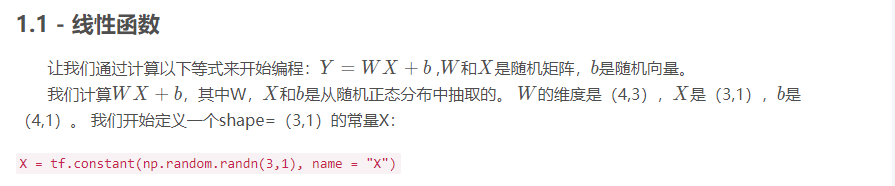
1.1 - Linear function 线性函数

你可能会发现以下功能有帮助:

·tf.matmul(…，…)来做一个矩阵乘法 #matmul 就是matrix和multiply
·tf.add(…，…)做加法
·随机初始化n .random.randn(…）

# GRADED FUNCTION: linear_function

def linear_function():
    """
    Implements a linear function: 
            Initializes W to be a random tensor of shape (4,3)
            Initializes X to be a random tensor of shape (3,1)
            Initializes b to be a random tensor of shape (4,1)
    Returns: 
    result -- runs the session for Y = WX + b 
    """
    
    np.random.seed(1)
    
    ### START CODE HERE ### (4 lines of code)
    X = tf.constant(np.random.randn(3, 1), name = 'X')
    W = tf.constant(np.random.randn(4, 3), name = 'W')
    b = tf.constant(np.random.randn(4, 1), name = 'b')
    Y = tf.add((tf.matmul(W, X)), b)
    ### END CODE HERE ### 
    
    # Create the session using tf.Session() and run it with sess.run(...) on the variable you want to calculate
    
    ### START CODE HERE ###
    sess = tf.compat.v1.Session()
    result = sess.run(Y)
    ### END CODE HERE ### 
    
    # close the session 
    sess.close()

    return result

# GRADED FUNCTION: linear_function

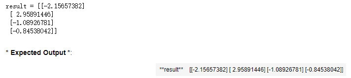
print( "result = " + str(linear_function()))

运行结果：

1.2 - Computing the sigmoid 计算sigmoid

太棒了!你只是实现了一个线性函数。Tensorflow提供了各种常用的神经网络函数，比如tf.sigmoid和tf.softmax。在这个练习中，我们计算输入的sigmoid函数。

在这个练习中，您必须

(i)创建一个占位符x，

(ii)定义使用tf计算sigmoid所需的操作。

(iii)运行会话。

练习**:实现下面的sigmoid函数。你应该使用以下方法:

tf.placeholder(tf.float32, name = "...")

tf.sigmoid(...)

sess.run(..., feed_dict = {x: z})

注意，在tensorflow中有两种典型的创建和使用会话的方法:

Method 1:

sess = tf.Session()
# Run the variables initialization (if needed), run the operations
result = sess.run(..., feed_dict = {...})
sess.close() # Close the session

Method 2:

with tf.Session() as sess: 
    # run the variables initialization (if needed), run the operations
    result = sess.run(..., feed_dict = {...})
    # This takes care of closing the session for you :)

# GRADED FUNCTION: sigmoid

def sigmoid(z):
    """
    Computes the sigmoid of z
    
    Arguments:
    z -- input value, scalar or vector
    
    Returns: 
    results -- the sigmoid of z
    """
    
    ### START CODE HERE ### ( approx. 4 lines of code)
    # Create a placeholder for x. Name it 'x'.
    x = tf.compat.v1.placeholder(tf.float32, name= 'x')

    # compute sigmoid(x)
    sigmoid = tf.sigmoid(x)

    # Create a session, and run it. Please use the method 2 explained above. 
    # You should use a feed_dict to pass z's value to x. 
    with tf.compat.v1.Session() as sess:
        # Run session and call the output "result"
        result = sess.run(sigmoid, feed_dict = {x : z})
    
    ### END CODE HERE ###
    
    return result

# GRADED FUNCTION: sigmoid

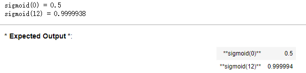
print ("sigmoid(0) = " + str(sigmoid(0)))
print ("sigmoid(12) = " + str(sigmoid(12)))

运行结果：

总结一下，你如何知道如何去**:

1、创建占位符。

2、指定与要计算的操作对应的计算图。

3、创建会话

4、运行会话，必要时使用feed字典指定占位符变量的值。

1.3 - Computing the Cost 计算成本

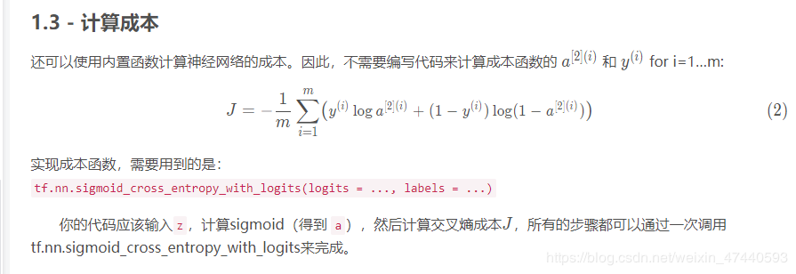
you can do it in one line of code in tensorflow!

练习:实现交叉熵损失。您将使用的函数是:

tf.nn.sigmoid_cross_entropy_with_logits(logits = ..., labels = ...)

 1 # GRADED FUNCTION: cost
 2 
 3 def cost(logits, labels):
 4     """
 5     Computes the cost using the sigmoid cross entropy
 6     
 7     Arguments:
 8     logits -- vector containing z, output of the last linear unit (before the final sigmoid activation)
 9                   包含z的向量，最后一个线性单元的输出(在最后的s型激活之前)
10     labels -- vector of labels y (1 or 0)  标签向量y
11     
12     Note: What we've been calling "z" and "y" in this class are respectively called "logits" and "labels" 
13     in the TensorFlow documentation. So logits will feed into z, and labels into y. 
14   注意:我们在这个类中所称的“z”和“y”分别称为“logits”和“label”
15     在TensorFlow文档中。所以logits会被输入z, label会被输入y。  
16     Returns:
17     cost -- runs the session of the cost (formula (2))
18     """
19     
20     ### START CODE HERE ### 
21     
22     # Create the placeholders for "logits" (z) and "labels" (y) (approx. 2 lines)
23     z = tf.compat.v1.placeholder(tf.float32, name = 'z')
24     y = tf.compat.v1.placeholder(tf.float32, name = 'y')
25     
26     # Use the loss function (approx. 1 line)
27     cost = tf.nn.sigmoid_cross_entropy_with_logits(logits = z, labels = y)
28     
29     # Create a session (approx. 1 line). See method 1 above.
30     sess = tf.compat.v1.Session()
31     
32     # Run the session (approx. 1 line).
33     cost = sess.run(cost, feed_dict = {z:logits, y:labels})#使用feed字典来输入，用z去喂logits，用y去喂label
34     
35     # Close the session (approx. 1 line). See method 1 above.
36     sess.close()
37     
38     ### END CODE HERE ###
39     
40     return cost

# GRADED FUNCTION: cost

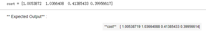
logits = sigmoid(np.array([0.2,0.4,0.7,0.9]))
cost = cost(logits, np.array([0,0,1,1]))
print ("cost = " + str(cost))

运行结果：

1.4 - Using One Hot encodings 使用独热编码（0、1编码）

在深度学习中，很多时候你会得到一个数字从0到C-1的y向量，其中C是类别的数量。如果C是样本数4，那么你可能有以下y向量，你将需要转换如下:

这被称为“one hot”编码，因为在转换后的表示中，每列中只有一个元素是“hot”(即设置为1)。在tensorflow中，你可以使用一行代码:

tf.one_hot(labels, depth, axis)

练习:执行下面的函数取一个向量的标签和类𝐶的总数,并返回一个独热编码。使用tf.one_hot()来完成此操作。

 1 # GRADED FUNCTION: one_hot_matrix
 2 
 3 def one_hot_matrix(labels, C):
 4     """
 5     Creates a matrix where the i-th row corresponds to the ith class number and the jth column
 6                      corresponds to the jth training example. So if example j had a label i. Then entry (i,j) 
 7                      will be 1.     创建一个矩阵，其中第i行对应第i个类号，第j列对应第j个训练样本    
 8                                     所以如果第j个样本对应着第i个标签，那么entry (i,j)将会是1
 9                      
10     Arguments:
11     labels -- vector containing the labels           lables - 标签向量
12     C -- number of classes, the depth of the one hot dimension          C - 分类数 一个热维度的深度
13     
14     Returns: 
15     one_hot -- one hot matrix 一个热矩阵
16     """
17     
18     ### START CODE HERE ###
19     
20     # Create a tf.constant equal to C (depth), name it 'C'. (approx. 1 line)
21     C = tf.constant(C, name = 'C')
22     
23     # Use tf.one_hot, be careful with the axis (approx. 1 line)
24     one_hot_matrix = tf.one_hot(labels, C, axis = 0)#这里是初始化，第一、二个参数都是靠形参来说输入的
25     
26     # Create the session (approx. 1 line)
27     sess = tf.compat.v1.Session()
28     
29     # Run the session (approx. 1 line)
30     one_hot = sess.run(one_hot_matrix)#为啥这里不用喂数据呢？数据靠形参输入的；run一下返回的是一个矩阵
31     
32     # Close the session (approx. 1 line). See method 1 above.
33     sess.close()
34     
35     ### END CODE HERE ###
36     
37     return one_hot

# GRADED FUNCTION: one_hot_matrix

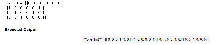
labels = np.array([1,2,3,0,2,1])
one_hot = one_hot_matrix(labels, C = 4)
print ("one_hot = " + str(one_hot))

运行结果：

1.5 - Initialize with zeros and ones 初始化0和1

现在您将学习如何初始化一个由0和1组成的向量。您将要调用的函数是tf.ones()。要用零进行初始化，可以使用tf.zeros()。这些函数采用一个形状，并分别返回一个充满0和1的维形数组。

练习:实现下面的函数以获取一个形状并返回一个数组(形状的维数为1)。

tf.ones(shape)

 1 # GRADED FUNCTION: ones
 2 
 3 def ones(shape):
 4     """
 5     Creates an array of ones of dimension shape     创建一个维度为shape的变量（数组），其值全为1
 6     
 7     Arguments:
 8     shape -- shape of the array you want to create 你要创建的数组的维度
 9         
10     Returns: 
11     ones -- array containing only ones 只包含1的数组   
12     """
13     
14     ### START CODE HERE ###
15     
16     # Create "ones" tensor using tf.ones(...). (approx. 1 line)
17     ones = tf.ones(shape)
18     
19     # Create the session (approx. 1 line)
20     sess = tf.compat.v1.Session()
21     
22     # Run the session to compute 'ones' (approx. 1 line)
23     ones = sess.run(ones)
24     
25     # Close the session (approx. 1 line). See method 1 above.
26     sess.close()
27     
28     ### END CODE HERE ###
29     return ones

# GRADED FUNCTION: ones

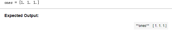
print ("ones = " + str(ones([3])))

运行结果：

2 - Building your first neural network in tensorflow 使用TensorFlow构建你的第一个神经网络

在作业的这一部分中，您将使用tensorflow构建一个神经网络。记住，实现tensorflow模型有两个部分:

·创建计算图
·运行图表

让我们钻研一下你想解决的问题吧!

2.0 - Problem statement: SIGNS Dataset 问题陈诉：符号数据集

一天下午，我们和一些朋友决定教我们的电脑破译手语。我们花了几个小时在一面白墙前拍照，并得到了以下数据集。现在你的工作是建立一种算法来促进语言障碍的人与不懂手语的人之间的交流。

训练集：有从0到5的数字的1080张图片(64x64像素)，每个数字拥有180张图片。

测试集：有从0到5的数字的120张图片(64x64像素)，每个数字拥有5张图片。

注意，这是符号数据集的一个子集。完整的数据集包含更多的符号。

下面是每个数字的样本，以及我们如何表示标签的解释。这些都是原始图片，我们实际上用的是64 * 64像素的图片。

Figure 1: SIGNS dataset

首先我们需要加载数据集：

# Loading the dataset 加载数据集
X_train_orig, Y_train_orig, X_test_orig, Y_test_orig, classes = load_dataset()

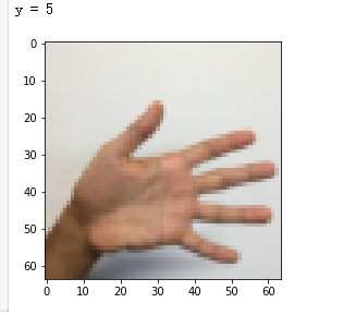
更改下面的索引并运行单元格以在数据集中显示一些示例。

# Example of a picture
index = 0
plt.imshow(X_train_orig[index])
print ("y = " + str(np.squeeze(Y_train_orig[:, index])))

运行结果：

和往常一样，我们要对数据集进行扁平化，然后再除以255以归一化数据，除此之外，我们要需要把每个标签转化为独热向量，像上面的图一样。

# Flatten the training and test images  扁平化
X_train_flatten = X_train_orig.reshape(X_train_orig.shape[0], -1).T  #这里的-1被理解为unspecified value，意思是未指定为给定的
X_test_flatten = X_test_orig.reshape(X_test_orig.shape[0], -1).T
# Normalize image vectors  归一化
X_train = X_train_flatten/255.
X_test = X_test_flatten/255.
# Convert training and test labels to one hot matrices 转化为独热矩阵
Y_train = convert_to_one_hot(Y_train_orig, 6)
Y_test = convert_to_one_hot(Y_test_orig, 6)

print ("number of training examples = " + str(X_train.shape[1]))
print ("number of test examples = " + str(X_test.shape[1]))
print ("X_train shape: " + str(X_train.shape))
print ("Y_train shape: " + str(Y_train.shape))
print ("X_test shape: " + str(X_test.shape))
print ("Y_test shape: " + str(Y_test.shape))

运行结果：

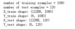
注意12288来自64×64×3。每个图像是正方形的，64×64像素，3是RGB颜色。在继续之前，请确保所有这些形状对你有意义。

您的目标是建立一种能够高精度识别符号的算法。为此，您将构建一个tensorflow模型，该模型与之前在numpy中构建的用于猫识别的模型几乎相同(但现在使用softmax输出)。现在是比较numpy实现和tensorflow实现的好时机。

模型为LINEAR -> RELU -> LINEAR -> RELU -> LINEAR -> SOFTMAX。SIGMOID输出层已转换为SOFTMAX。SOFTMAX层将SIGMOID泛化到有两个以上的类时。

2.1 - Create placeholders 创建占位符

您的第一个任务是为X和y创建占位符，这将允许您在稍后运行会话时传入训练数据。

练习:实现下面的函数在tensorflow中创建占位符。

 1 # GRADED FUNCTION: create_placeholders
 2 
 3 def create_placeholders(n_x, n_y):
 4     """
 5     Creates the placeholders for the tensorflow session.     为TensorFlow会话创建占位符
 6     
 7     Arguments:
 8     n_x -- scalar, size of an image vector (num_px * num_px = 64 * 64 * 3 = 12288) 一个实数，图片向量的大小（64*64*3 = 12288）
 9     n_y -- scalar, number of classes (from 0 to 5, so -> 6) 一个实数，分类数（从0到5，所以n_y = 6）
10     
11     Returns:
12     X -- placeholder for the data input, of shape [n_x, None] and dtype "float" 一个数据输入的占位符，维度为[n_x, None]，dtype = "float"
13     Y -- placeholder for the input labels, of shape [n_y, None] and dtype "float"一个对应输入的标签的占位符，维度为[n_y,None]，dtype = "float"
14     
15     Tips:
16     - You will use None because it let's us be flexible on the number of examples you will for the placeholders.
17       In fact, the number of examples during test/train is different.
18     使用None，因为它让我们可以灵活处理占位符提供的样本数量。事实上，测试/训练期间的样本数量是不同的。
19     """
20     ### START CODE HERE ### (approx. 2 lines)
21     X = tf.compat.v1.placeholder(dtype = tf.float32, shape = [n_x, None]) ##这里注意下tf版本，和原博客不一致
22     Y = tf.compat.v1.placeholder(dtype = tf.float32, shape = [n_y, None])
23     ### END CODE HERE ###
24     
25     return X, Y

# GRADED FUNCTION: create_placeholders

X, Y = create_placeholders(12288, 6)
print ("X = " + str(X))
print ("Y = " + str(Y))

运行结果：

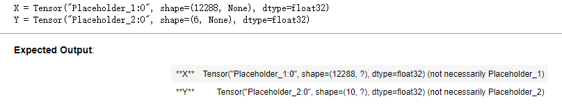
这边输出的第一个参数为名字，因为没有设置name，反复运行的话，1:0这里 1是会改变的，表示的是分配必要的内存，每次的内存不一样。

2.2 - Initializing the parameters 初始化参数

第二个任务是初始化tensorflow中的参数。

练习:实现下面的函数来初始化tensorflow中的参数。你要用Xavier初始化权重和用零初始化偏差。形状如下所示。举个例子，为了帮助你，对于W1和b1你可以使用:

W1 = tf.get_variable("W1", [25,12288], initializer = tf.contrib.layers.xavier_initializer(seed = 1))
b1 = tf.get_variable("b1", [25,1], initializer = tf.zeros_initializer())

Please use seed = 1 to make sure your results match ours.

原博文报错：

①AttributeError: module 'tensorflow' has no attribute 'reset_default_graph'

解决办法：将tf.reset_default_graph() 改为 ops.reset_default_graph()

②AttributeError: module 'tensorflow' has no attribute 'set_random_seed'

解决方法：module 'tensorflow' has no attribute 'set_random_seed'，将tf.set_random_seed(1) 改为 tf.random.set_seed(1) 本人是tf2.0版本

③AttributeError: module 'tensorflow' has no attribute 'contrib'

由于TF2.x删除了contrib，我使用了initializer = tf.initializers.GlorotUniform(seed=1))来代替initializer=tf.contrib.layers.xavier_initializer(seed=1))

 1 # GRADED FUNCTION: initialize_parameters
 2 
 3 def initialize_parameters():
 4     """
 5     Initializes parameters to build a neural network with tensorflow. The shapes are: 初始化神经网络的参数，参数的维度如下：
 6                         W1 : [25, 12288]
 7                         b1 : [25, 1]
 8                         W2 : [12, 25]
 9                         b2 : [12, 1]
10                         W3 : [6, 12]
11                         b3 : [6, 1]
12     
13     Returns:
14     parameters -- a dictionary of tensors containing W1, b1, W2, b2, W3, b3  包含了W和b的字典
15     """
16     
17 #     tf.set_random_seed(1)                   # so that your "random" numbers match ours
18     tf.random.set_seed(1)       
19     
20     ### START CODE HERE ### (approx. 6 lines of code)
21 #   W1 = tf.compat.v1.get_variable('W1', [25, 12288], initializer = tf.contrib.layers.xavier_initializer(seed = 1))
22     W1 = tf.compat.v1.get_variable("W1",[25,12288],initializer = tf.initializers.GlorotUniform(seed=1))
23     b1 = tf.compat.v1.get_variable('b1', [25, 1], initializer = tf.zeros_initializer())
24 #   W2 = tf.compat.v1.get_variable('W2', [12, 25], initializer = tf.contrib.layers.xavier_initializer(seed = 1))
25     W2 = tf.compat.v1.get_variable("W2", [12, 25], initializer = tf.initializers.GlorotUniform(seed=1))
26     b2 = tf.compat.v1.get_variable('b2', [12, 1], initializer = tf.zeros_initializer())
27 #   W3 = tf.compat.v1.get_variable('W3', [6, 1], initializer = tf.contrib.layers.xavier_initializer(seed = 1))
28     W3 = tf.compat.v1.get_variable("W3", [6, 12], initializer = tf.initializers.GlorotUniform(seed=1))
29     b3 = tf.compat.v1.get_variable('b3', [6, 1], initializer = tf.zeros_initializer())
30 
31     ### END CODE HERE ###
32 
33     parameters = {"W1": W1,
34                   "b1": b1,
35                   "W2": W2,
36                   "b2": b2,
37                   "W3": W3,
38                   "b3": b3}
39     
40     return parameters

# GRADED FUNCTION: initialize_parameters

# tf.reset_default_graph() #用于清除默认图形堆栈并重置全局默认图形  由于本次使用的TF框架是2.x的原因 更改为：
ops.reset_default_graph() #用于清除默认图形堆栈并重置全局默认图形。 
with tf.compat.v1.Session() as sess:
    parameters = initialize_parameters()
    print("W1 = " + str(parameters["W1"]))
    print("b1 = " + str(parameters["b1"]))
    print("W2 = " + str(parameters["W2"]))
    print("b2 = " + str(parameters["b2"]))

运行结果：

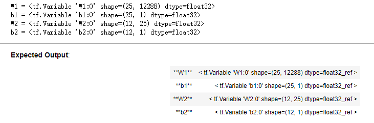
正如预期的那样，还没有对参数进行计算。

2.3 - Forward propagation in tensorflow TensorFlow中的前向传播

现在您将在tensorflow中实现前向传播模块。该函数将接受一个参数字典，并完成前向传递。您将使用的功能是:

tf.add(...,...) to do an addition 加法

tf.matmul(...,...) to do a matrix multiplication 矩阵乘法

tf.nn.relu(...) to apply the ReLU activation 应用relu激活函数

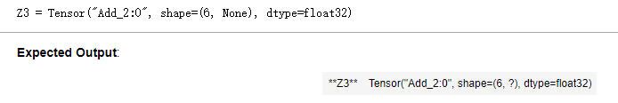
问题:实现神经网络的前向传递。我们为您注释了对应的numpy，以便您可以比较tensorflow实现和numpy。值得注意的是，正向传播在z3停止。原因是在tensorflow中，最后的线性层输出被作为函数的输入来计算损失。因此，您不需要a3!

 1 # GRADED FUNCTION: forward_propagation
 2 
 3 def forward_propagation(X, parameters):
 4     """
 5     Implements the forward propagation for the model: LINEAR -> RELU -> LINEAR -> RELU -> LINEAR -> SOFTMAX
 6         实现一个模型的前向传播，模型结构为LINEAR -> RELU -> LINEAR -> RELU -> LINEAR -> SOFTMAX
 7     Arguments:
 8     X -- input dataset placeholder, of shape (input size, number of examples) 输入数据的占位符，维度为（输入节点数量，样本数量）
 9     parameters -- python dictionary containing your parameters "W1", "b1", "W2", "b2", "W3", "b3" 包含了W和b的参数的字典
10                   the shapes are given in initialize_parameters
11 
12     Returns:
13     Z3 -- the output of the last LINEAR unit 最后一个LINEAR节点的输出
14     """
15     
16     # Retrieve the parameters from the dictionary "parameters"  从字典“parameters”检索参数
17     W1 = parameters['W1']
18     b1 = parameters['b1']
19     W2 = parameters['W2']
20     b2 = parameters['b2']
21     W3 = parameters['W3']
22     b3 = parameters['b3']
23     
24     ### START CODE HERE ### (approx. 5 lines)              # Numpy Equivalents:
25     Z1 = tf.add(tf.matmul(W1, X), b1)                      # Z1 = np.dot(W1, X) + b1
26     #Z1 = tf.matmul(W1,X) + b1             #也可以这样写
27     A1 = tf.nn.relu(Z1)                                    # A1 = relu(Z1)
28     Z2 = tf.add(tf.matmul(W2, A1), b2)                     # Z2 = np.dot(W2, a1) + b2
29     A2 = tf.nn.relu(Z2)                                    # A2 = relu(Z2)
30     Z3 = tf.add(tf.matmul(W3, A2), b3)                     # Z3 = np.dot(W3,Z2) + b3
31     ### END CODE HERE ###
32     
33     return Z3

# GRADED FUNCTION: forward_propagation

# tf.reset_default_graph()  #用于清除默认图形堆栈并重置全局默认图形。由于使用tf2.0版本，这个不适用
ops.reset_default_graph()
with tf.compat.v1.Session() as sess:
    X, Y = create_placeholders(12288, 6)
    parameters = initialize_parameters()
    Z3 = forward_propagation(X, parameters)
    print("Z3 = " + str(Z3))

运行结果：

您可能已经注意到，正向传播不输出任何缓存。当我们讲到brackpropagation的时候，你就会明白为什么了。

2.4 Compute cost 计算成本

如前所见，很容易计算成本使用:

tf.reduce_mean(tf.nn.softmax_cross_entropy_with_logits(logits = ..., labels = ...))

问题:执行下面的成本函数。

了解tf.nn.softmax_cross_entropy_with_logits的“logits”和“labels”输入是被期望为形状（样本数，分类数）是很重要的。这样我们就把Z3和Y转置了。

此外,tf.reduce_mean基本上是对例子进行总结。

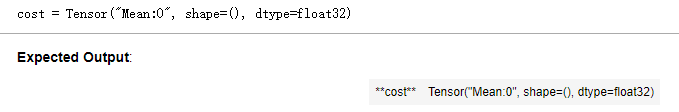
 1 # GRADED FUNCTION: compute_cost 
 2 
 3 def compute_cost(Z3, Y):
 4     """
 5     Computes the cost 计算成本
 6     
 7     Arguments:
 8     Z3 -- output of forward propagation (output of the last LINEAR unit), of shape (6, number of examples) 前向传播的结果
 9     Y -- "true" labels vector placeholder, same shape as Z3 标签，一个占位符，和Z3的维度相同
10     
11     Returns:
12     cost - Tensor of the cost function 成本函数的值
13     """
14     
15     # to fit the tensorflow requirement for tf.nn.softmax_cross_entropy_with_logits(...,...)
16     logits = tf.transpose(Z3) #转置
17     labels = tf.transpose(Y)
18     
19     ### START CODE HERE ### (1 line of code)
20     cost = tf.reduce_mean(tf.nn.softmax_cross_entropy_with_logits(logits = logits, labels = labels))
21     ### END CODE HERE ###
22     
23     return cost

# GRADED FUNCTION: compute_cost

# tf.reset_default_graph()
ops.reset_default_graph() #用于清除默认图形堆栈并重置全局默认图形。

with tf.compat.v1.Session() as sess:
    X, Y = create_placeholders(12288, 6)
    parameters = initialize_parameters()
    Z3 = forward_propagation(X, parameters)
    cost = compute_cost(Z3, Y)
    print("cost = " + str(cost))

运行结果：

2.5 - Backward propagation & parameter updates 反向传播&参数更新

这就是你感激编程框架的地方。所有的反向传播和参数更新都在一行代码中完成。在模型中加入这条线是很容易的。

在计算成本函数之后。您将创建一个“optimizer”对象。在运行tf.session时，必须调用该对象以及成本。当被调用时，它将使用所选的方法和学习率对给定的代价进行优化。

例如，对于梯度下降优化器将是:

optimizer = tf.train.GradientDescentOptimizer(learning_rate = learning_rate).minimize(cost）

为了做到优化，你会这样做:

_ , c = sess.run([optimizer, cost], feed_dict={X: minibatch_X, Y: minibatch_Y})

这通过以相反的顺序穿过tensorflow图来计算反向传播。从成本到输入。

注意，在编码时，我们经常使用‘_’作为一个“一次性”变量来存储我们以后不需要使用的值。在这里，‘_’接受优化器的计算值，这是我们不需要的(而c取值为成本变量的值)。

2.6 - Building the model 建立模型

现在，你要把它们结合在一起!

练习:实现模型。您将调用之前实现的函数。

  1 def model(X_train, Y_train, X_test, Y_test, learning_rate = 0.0001,
  2           num_epochs = 1500, minibatch_size = 32, print_cost = True, is_plot = True):
  3     """
  4     Implements a three-layer tensorflow neural network: LINEAR->RELU->LINEAR->RELU->LINEAR->SOFTMAX.
  5         实现一个三层的TensorFlow神经网络：LINEAR->RELU->LINEAR->RELU->LINEAR->SOFTMAX
  6         
  7     Arguments:
  8     X_train -- training set, of shape (input size = 12288, number of training examples = 1080) 
  9     训练集，维度为（输入大小（输入节点数量） = 12288, 样本数量 = 1080）
 10     
 11     Y_train -- test set, of shape (output size = 6, number of training examples = 1080)
 12     训练集分类数量，维度为（输出大小(输出节点数量) = 6, 样本数量 = 1080）
 13     
 14     X_test -- training set, of shape (input size = 12288, number of training examples = 120)
 15     测试集，维度为（输入大小（输入节点数量） = 12288, 样本数量 = 120）
 16     
 17     Y_test -- test set, of shape (output size = 6, number of test examples = 120)
 18     测试集分类数量，维度为（输出大小(输出节点数量) = 6, 样本数量 = 120）
 19     
 20     learning_rate -- learning rate of the optimization  学习速率，
 21     num_epochs -- number of epochs of the optimization loop 整个训练集的遍历次数
 22     minibatch_size -- size of a minibatch  每个小批量数据集的大小
 23     print_cost -- True to print the cost every 100 epochs 是否打印成本，每100代打印一次
 24     is_plot - 是否绘制曲线图
 25     
 26     Returns:
 27     parameters -- parameters learnt by the model. They can then be used to predict. 学习后的参数，然后可以用作预测
 28     """
 29     
 30     ops.reset_default_graph()                         # to be able to rerun the model without overwriting tf variables
 31     #能够重新运行模型而不覆盖tf变量
 32     
 33 #     tf.set_random_seed(1)                             # to keep consistent results
 34     tf.random.set_seed(1)
 35     seed = 3                                          # to keep consistent results
 36     (n_x, m) = X_train.shape                          # (n_x: input size, m : number of examples in the train set) 获取输入节点数量和样本数
 37     n_y = Y_train.shape[0]                            # n_y : output size 获取输出节点数量
 38     costs = []                                        # To keep track of the cost 保持对成本的追踪
 39     
 40     #要用到之前创建好的函数
 41     # Create Placeholders of shape (n_x, n_y) 给X和Y创建placeholder
 42     ### START CODE HERE ### (1 line)
 43     X, Y = create_placeholders(n_x, n_y)
 44     ### END CODE HERE ###
 45 
 46     # Initialize parameters 初始化参数
 47     ### START CODE HERE ### (1 line)
 48     parameters = initialize_parameters()
 49     ### END CODE HERE ###
 50     
 51     # Forward propagation: Build the forward propagation in the tensorflow graph
 52     ### START CODE HERE ### (1 line)
 53     Z3 = forward_propagation(X, parameters)
 54     ### END CODE HERE ###
 55     
 56     # Cost function: Add cost function to tensorflow graph
 57     ### START CODE HERE ### (1 line)
 58     cost = compute_cost(Z3, Y)
 59     ### END CODE HERE ###
 60     
 61     # Backpropagation: Define the tensorflow optimizer. Use an AdamOptimizer.反向传播，使用Adam优化
 62     ### START CODE HERE ### (1 line)
 63     optimizer = tf.compat.v1.train.AdamOptimizer(learning_rate = learning_rate).minimize(cost)
 64     ### END CODE HERE ###
 65     
 66     # Initialize all the variables 初始化所有的变量
 67     init = tf.compat.v1.global_variables_initializer()
 68 
 69     # Start the session to compute the tensorflow graph 开始会话并计算tensorflow图
 70     with tf.compat.v1.Session() as sess:
 71         
 72         # Run the initialization 初始化
 73         sess.run(init)
 74         
 75         # Do the training loop
 76         for epoch in range(num_epochs):
 77 
 78             epoch_cost = 0.                       # Defines a cost related to an epoch 定义一个每代的成本
 79             num_minibatches = int(m / minibatch_size) # number of minibatches of size minibatch_size in the train set  minibatch的总数量
 80             seed = seed + 1
 81             minibatches = random_mini_batches(X_train, Y_train, minibatch_size, seed)  #原代码
 82 #             minibatches = tf_utils.random_mini_batches(X_train, Y_train, minibatch_size, seed) #参考的代码
 83             for minibatch in minibatches:
 84 
 85                 # Select a minibatch 选择一个minibatch
 86                 (minibatch_X, minibatch_Y) = minibatch
 87                 
 88                 # IMPORTANT: The line that runs the graph on a minibatch. 重要：在一个小批处理上运行图形的线。
 89                 # Run the session to execute the "optimizer" and the "cost", the feed_dict should contain a minibatch for (X,Y).
 90                 #为了执行“优化器”和“成本”，feed_dict应该包含一个针对(X,Y)的小批处理。
 91                 ### START CODE HERE ### (1 line)
 92                 _ , minibatch_cost = sess.run([optimizer, cost], feed_dict = {X : minibatch_X, Y : minibatch_Y})
 93                 ### END CODE HERE ###
 94                 
 95                 #计算这个minibatch在这一代中所占的误差
 96                 epoch_cost += minibatch_cost / num_minibatches
 97                 
 98                
 99             # Print the cost every epoch 每一个epoch都打印成本
100             if print_cost == True and epoch % 100 == 0:
101                 print ("Cost after epoch %i: %f" % (epoch, epoch_cost))
102             if print_cost == True and epoch % 5 == 0:
103                 costs.append(epoch_cost)
104                 
105         # plot the cost 这边自己修改成可请求的
106         if is_plot:
107             plt.plot(np.squeeze(costs))
108             plt.ylabel('cost')
109             plt.xlabel('iterations (per tens)')
110             plt.title("Learning rate =" + str(learning_rate))
111             plt.show()
112 
113         # lets save the parameters in a variable  保存学习后的参数在一个变量里
114         parameters = sess.run(parameters)
115         print ("Parameters have been trained!")
116 
117         # Calculate the correct predictions 计算当前的预测结果
118         correct_prediction = tf.equal(tf.argmax(Z3), tf.argmax(Y))
119 
120         # Calculate accuracy on the test set 计算测试集的准确率  mean是平均值的意思？
121         accuracy = tf.reduce_mean(tf.cast(correct_prediction, "float"))
122 
123         print ("Train Accuracy:", accuracy.eval({X: X_train, Y: Y_train}))
124         print ("Test Accuracy:", accuracy.eval({X: X_test, Y: Y_test}))
125         
126         return parameters

实现我们的模型

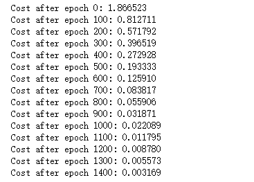
import time
#开始时间
start_time = time.perf_counter() 
#开始训练
parameters = model(X_train, Y_train, X_test, Y_test)
#结束时间
end_time = time.perf_counter() 
#计算时差
print("CPU的执行时间 = " + str(end_time - start_time) + " 秒" )

运行结果：

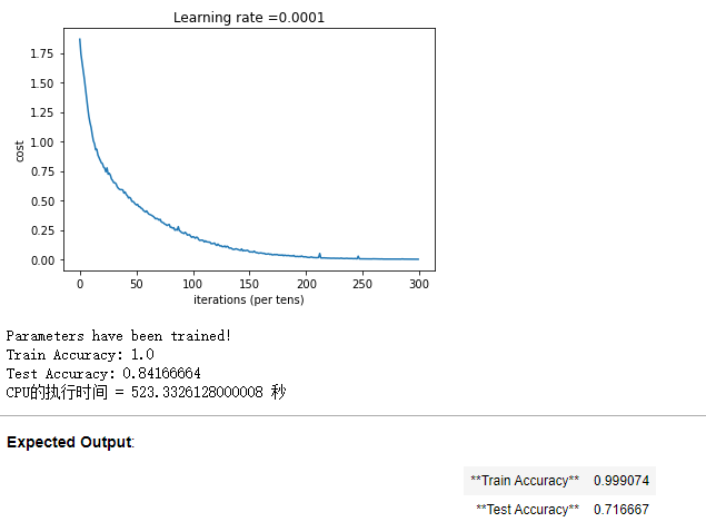
令人惊讶的是，您的算法能够识别表示0到5之间数字的符号，准确率为71.7%。

见解:

你的模型看起来足够大，可以很好地适应训练集。然而，考虑到训练和测试精度之间的差异，你可以尝试增加L2或放弃正则化来减少过拟合。
可以将会话看作是训练模型的代码块。每次在迷你批处理上运行会话时，它都会训练参数。总的来说，您已经运行了会话很多次(1500个epoch)，直到您获得了经过良好训练的参数。

2.7 - Test with your own image (optional / ungraded exercise) 测试你自己的图片（选做）

恭喜你完成了这项任务。您现在可以拍摄您的手的照片，并看到您的模型的输出。要做到这一点:

1、点击这个笔记本上面一栏的“文件”，然后点击“打开”进入你的Coursera中心。

2、将您的图像添加到此Jupyter Notebook的目录，在“images”文件夹

3、将图像名称写入以下代码4。运行代码并检查算法是否正确!

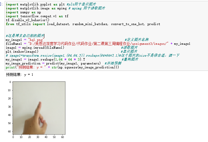
博主自己拍了5张图片，然后裁剪成1：1的样式，再通过格式工厂把很大的图片缩放成64x64的图片，同时把jpg转化为png，因为mpimg只能读取png的图片。

 1 import matplotlib.pyplot as plt #plt用于显示图片
 2 import matplotlib.image as mpimg # mpimg 用于读取图片
 3 import numpy as np
 4 import tensorflow.compat.v1 as tf
 5 tf.disable_v2_behavior()
 6 from tf_utils import load_dataset, random_mini_batches, convert_to_one_hot, predict
 7 
 8 
 9 #这是博主自己拍的图片
10 my_image1 = "hq_thumbs_up.png"                                            #定义图片名称
11 fileName1 = "D:/吴恩达深度学习代码作业/代码作业/第二课第三周编程作业/assignment3/images/" + my_image1                      #图片地址
12 image1 = mpimg.imread(fileName1)                               #读取图片
13 plt.imshow(image1)                                             #显示图片
14 # image1=transform.resize(image1,(64,64,3)).reshape(64*64*3,1)#这个图片的size不是很合适，调一下
15 my_image1 = image1.reshape(1,64 * 64 * 3).T                    #重构图片
16 my_image_prediction = predict(my_image1, parameters)  #开始预测
17 print("预测结果: y = " + str(np.squeeze(my_image_prediction)))

预测竖起大拇指

运行结果：

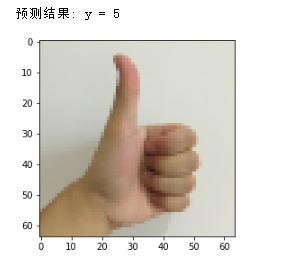
改变图片，

2.5 - Backward propagation & parameter updates

posted @ 2020-08-21 09:07 廖海清阅读(1428) 评论(2) 编辑收藏举报

会员力量，点亮园子希望

刷新页面返回顶部

Agiroy_70's Blog

吴恩达深度学习第二课第三周编程作业_TensorFlow Tutorial TensorFlow教程

TensorFlow Tutorial TensorFlow教程

1 - Exploring the Tensorflow Library 探索Tensorflow库

1.1 - Linear function 线性函数

1.2 - Computing the sigmoid 计算sigmoid

1.3 - Computing the Cost 计算成本

1.4 - Using One Hot encodings 使用独热编码（0、1编码）

1.5 - Initialize with zeros and ones 初始化0和1

2 - Building your first neural network in tensorflow 使用TensorFlow构建你的第一个神经网络

2.0 - Problem statement: SIGNS Dataset 问题陈诉：符号数据集

2.1 - Create placeholders 创建占位符

2.2 - Initializing the parameters 初始化参数

2.3 - Forward propagation in tensorflow TensorFlow中的前向传播

2.4 Compute cost 计算成本

2.5 - Backward propagation & parameter updates 反向传播&参数更新

2.6 - Building the model 建立模型

2.7 - Test with your own image (optional / ungraded exercise) 测试你自己的图片（选做）

2.5 - Backward propagation & parameter updates

公告

Agiroy_70's Blog

吴恩达深度学习 第二课第三周编程作业_TensorFlow Tutorial TensorFlow教程

TensorFlow Tutorial TensorFlow教程

1 - Exploring the Tensorflow Library 探索Tensorflow库

1.1 - Linear function 线性函数

1.2 - Computing the sigmoid 计算sigmoid

1.3 - Computing the Cost 计算成本

1.4 - Using One Hot encodings 使用独热编码（0、1编码）

1.5 - Initialize with zeros and ones 初始化0和1

2 - Building your first neural network in tensorflow 使用TensorFlow构建你的第一个神经网络

2.0 - Problem statement: SIGNS Dataset 问题陈诉：符号数据集

2.1 - Create placeholders 创建占位符

2.2 - Initializing the parameters 初始化参数

2.3 - Forward propagation in tensorflow TensorFlow中的前向传播

2.4 Compute cost 计算成本

2.5 - Backward propagation & parameter updates 反向传播&参数更新

2.6 - Building the model 建立模型

2.7 - Test with your own image (optional / ungraded exercise) 测试你自己的图片（选做）

2.5 - Backward propagation & parameter updates

公告

吴恩达深度学习第二课第三周编程作业_TensorFlow Tutorial TensorFlow教程