吴恩达深度学习第二课第一周编程作业_regularization（正则化）

Regularization 正则化

声明

本文作业是在jupyter notebook上一步一步做的，带有一些过程中查找的资料等（出处已标明）并翻译成了中文，如有错误，欢迎指正！

参考：https://blog.csdn.net/u013733326/article/details/79847918

参考Kulbear 的【Initialization】和【Regularization】和【Gradient Checking】，以及念师的【10. 初始化、正则化、梯度检查实战】，以及何宽，

欢迎来到本周的第二次作业。深度学习模型有很大的灵活性和容量，如果训练数据集不够大，过拟合可能会成为一个严重的问题。当然，它在训练集上做得很好，但学习过的网络不能推广到它从未见过的新例子!（也就是训练可以，一到实战测试就拉胯。）

　　第二个作业的目的：

　　2. 正则化模型：

　　　　2.1：使用二范数对二分类模型正则化，尝试避免过拟合。

　　　　2.2：使用随机删除节点的方法精简模型，同样是为了尝试避免过拟合。

您将学习:在您的深度学习模型中使用正则化。

让我们首先导入将要使用的包。

# import packages
import numpy as np
import matplotlib.pyplot as plt
from reg_utils import sigmoid, relu, plot_decision_boundary, initialize_parameters, load_2D_dataset, predict_dec
from reg_utils import compute_cost, predict, forward_propagation, backward_propagation, update_parameters
import sklearn
import sklearn.datasets
import scipy.io #scipy是构建在numpy的基础之上的，它提供了许多的操作numpy的数组的函数。scipy.io包提供了多种功能来解决不同格式的文件的输入和输出。
from testCases import *  #from XXX import*是把XXX下的所有名字引入当前名称空间。 

%matplotlib inline
plt.rcParams['figure.figsize'] = (7.0, 4.0) # set default size of plots
plt.rcParams['image.interpolation'] = 'nearest'
plt.rcParams['image.cmap'] = 'gray'

C:\Users\1\Downloads\代码作业\第二课第一周编程作业\assignment1\reg_utils.py:85: SyntaxWarning: assertion is always true, perhaps remove parentheses?
  assert(parameters['W' + str(l)].shape == layer_dims[l], layer_dims[l-1])
C:\Users\1\Downloads\代码作业\第二课第一周编程作业\assignment1\reg_utils.py:86: SyntaxWarning: assertion is always true, perhaps remove parentheses?
  assert(parameters['W' + str(l)].shape == layer_dims[l], 1)

scipy基础—io，来自：伏都哥哥，链接：https://blog.csdn.net/engerla/article/details/94332213

问题陈述：你刚刚被法国足球公司聘为AI专家。他们希望你能推荐法国队守门员应该在什么位置踢球，这样法国队的球员就可以用头去碰球了。

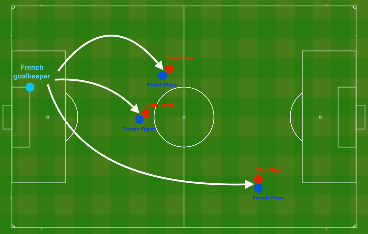
**Figure 1** : **Football field** 图一足球场

守门员把球踢向空中，每个队的队员都在拼命地用头击球

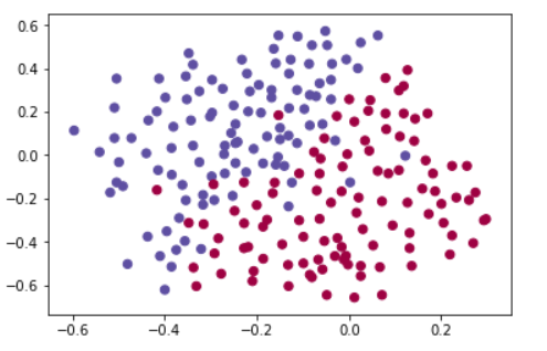
他们提供了以下来自法国过去10场比赛的2D数据集。

train_X, train_Y, test_X, test_Y = load_2D_dataset()

每个点对应足球场上法国守门员从球场左侧射门后，足球运动员用头击球的位置。
•如果圆点是蓝色的，表示法国球员用头击中了球
•如果圆点是红色的，表示对方队员用头击球

你的目标：使用深度学习模型来找到守门员应该在场上踢球的位置。

数据集的分析：这个数据集有点嘈杂，但是它看起来像一条对角线，将左上角(蓝色)和右下角(红色)分开，这样会很好。
您将首先尝试一个非正则化的模型。然后，您将学习如何将其规范化，并决定选择哪种模型来解决法国足球公司的问题。

1 - Non-regularized model 无正则化的模型

您将使用以下神经网络(下面已经为您实现)。该模型可以使用:
•正则化模式——通过设置lambd输入为一个非零值。我们使用“lambd”而不是“lambda”，因为“lambda”在Python中是一个保留关键字。
•dropout模式（随机删除节点）——通过设置keep_prob的值小于1

您将首先尝试不进行任何正则化的模型。然后，你将实现:
•L2正则化——函数:“compute_cost_with_regularization()”和“backward_propagation_with_regularization()”
•Dropout——函数:“forward_propagation_with_dropout()”和“backward_propagation_with_dropout()”

在每个部分中，您将使用正确的输入运行此模型，以便它调用已实现的函数。请查看下面的代码以熟悉模型。

 1 def model(X, Y, learning_rate = 0.3, num_iterations = 30000, print_cost = True, lambd = 0, keep_prob = 1):
 2     """
 3     Implements a three-layer neural network: LINEAR->RELU->LINEAR->RELU->LINEAR->SIGMOID.
 4     
 5     Arguments:
 6     X -- input data, of shape (input size, number of examples)输入的数据，维度为(2, 要训练/测试的数量)
 7     Y -- true "label" vector (1 for blue dot / 0 for red dot), of shape (output size, number of examples)
 8     learning_rate -- learning rate of the optimization
 9     num_iterations -- number of iterations of the optimization loop
10     print_cost -- If True, print the cost every 10000 iterations
11     lambd -- regularization hyperparameter, scalar 正则化超参数，标量
12     keep_prob - probability of keeping a neuron active during drop-out, scalar.在dropout过程中保持神经元活跃的概率，标量
13     
14     Returns:
15     parameters -- parameters learned by the model. They can then be used to predict.
16     """
17         
18     grads = {}
19     costs = []                            # to keep track of the cost 
20     m = X.shape[1]                        # number of examples
21     layers_dims = [X.shape[0], 20, 3, 1]
22     
23     # Initialize parameters dictionary.
24     parameters = initialize_parameters(layers_dims)
25 
26     # Loop (gradient descent)
27 
28     for i in range(0, num_iterations):
29 
30         # Forward propagation: LINEAR -> RELU -> LINEAR -> RELU -> LINEAR -> SIGMOID.
31         if keep_prob == 1:
32             a3, cache = forward_propagation(X, parameters)
33         elif keep_prob < 1: #使用上了dropout
34             a3, cache = forward_propagation_with_dropout(X, parameters, keep_prob)
35         
36         # Cost function 计算成本
37         if lambd == 0:
38             cost = compute_cost(a3, Y)
39         else:#使用上了L2正则化
40             cost = compute_cost_with_regularization(a3, Y, parameters, lambd)
41             
42         # Backward propagation.
43         assert(lambd==0 or keep_prob==1)    # it is possible to use both L2 regularization and dropout, 可以同时使用L2正则化和dropout，
44                                             # but this assignment will only explore one at a time 这次作业一次只探讨一个问题
45         if lambd == 0 and keep_prob == 1: #不使用L2正则化，也没使用dropout，就正常的反向传播
46             grads = backward_propagation(X, Y, cache)
47         elif lambd != 0: #只使用了L2正则化
48             grads = backward_propagation_with_regularization(X, Y, cache, lambd)
49         elif keep_prob < 1:#只使用了dropout
50             grads = backward_propagation_with_dropout(X, Y, cache, keep_prob)
51         
52         # Update parameters.参数更新
53         parameters = update_parameters(parameters, grads, learning_rate)
54         
55         # Print the loss every 10000 iterations
56         if print_cost and i % 10000 == 0:
57             print("Cost after iteration {}: {}".format(i, cost))
58         if print_cost and i % 1000 == 0:
59             costs.append(cost)
60     
61     # plot the cost
62     plt.plot(costs)
63     plt.ylabel('cost')
64     plt.xlabel('iterations (x1,000)')
65     plt.title("Learning rate =" + str(learning_rate))
66     plt.show()
67     
68     return parameters

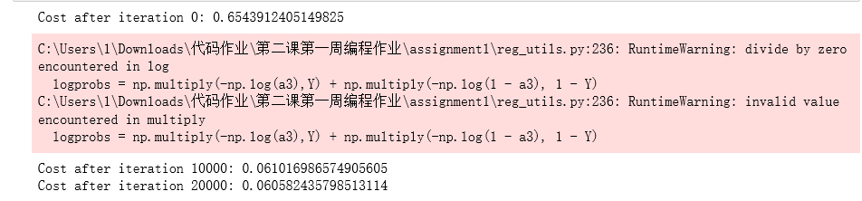
让我们在不进行任何正则化的情况下训练模型，并观察在训练/测试集上的准确性。

parameters = model(train_X, train_Y)
print ("On the training set:")
predictions_train = predict(train_X, train_Y, parameters)
print ("On the test set:")
predictions_test = predict(test_X, test_Y, parameters)

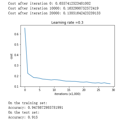
训练精度为94.8%，试验精度为91.5%。这是基线模型(您将观察正则化对该模型的影响)。运行以下代码以绘制模型的决策边界。

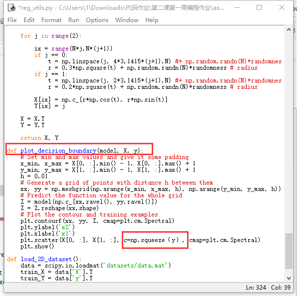
plt.title("Model without regularization")
axes = plt.gca()
axes.set_xlim([-0.75,0.40])
axes.set_ylim([-0.75,0.65])
plot_decision_boundary(lambda x: predict_dec(parameters, x.T), train_X, train_Y)

注意这里会报错：

TypeError                                 Traceback (most recent call last)
D:\ProgramData\Anaconda3\lib\site-packages\matplotlib\colors.py in to_rgba(c, alpha)
    165     try:
--> 166         rgba = _colors_full_map.cache[c, alpha]
    167     except (KeyError, TypeError):  # Not in cache, or unhashable.

TypeError: unhashable type: 'numpy.ndarray'

During handling of the above exception, another exception occurred:

ValueError                                Traceback (most recent call last)
D:\ProgramData\Anaconda3\lib\site-packages\matplotlib\axes\_axes.py in scatter(self, x, y, s, c, marker, cmap, norm, vmin, vmax, alpha, linewidths, verts, edgecolors, **kwargs)
   4287                 # must be acceptable as PathCollection facecolors
-> 4288                 colors = mcolors.to_rgba_array(c)
   4289             except ValueError:

D:\ProgramData\Anaconda3\lib\site-packages\matplotlib\colors.py in to_rgba_array(c, alpha)
    266     for i, cc in enumerate(c):
--> 267         result[i] = to_rgba(cc, alpha)
    268     return result

D:\ProgramData\Anaconda3\lib\site-packages\matplotlib\colors.py in to_rgba(c, alpha)
    167     except (KeyError, TypeError):  # Not in cache, or unhashable.
--> 168         rgba = _to_rgba_no_colorcycle(c, alpha)
    169         try:

D:\ProgramData\Anaconda3\lib\site-packages\matplotlib\colors.py in _to_rgba_no_colorcycle(c, alpha)
    222     if len(c) not in [3, 4]:
--> 223         raise ValueError("RGBA sequence should have length 3 or 4")
    224     if len(c) == 3 and alpha is None:

ValueError: RGBA sequence should have length 3 or 4

During handling of the above exception, another exception occurred:

ValueError                                Traceback (most recent call last)
<ipython-input-8-1c83d5b7143d> in <module>()
      3 axes.set_xlim([-0.75,0.40])
      4 axes.set_ylim([-0.75,0.65])
----> 5 plot_decision_boundary(lambda x: predict_dec(parameters, x.T), train_X, train_Y)

~\Downloads\代码作业\第二课第一周编程作业\assignment1\reg_utils.py in plot_decision_boundary(model, X, y)
    322     plt.ylabel('x2')
    323     plt.xlabel('x1')
--> 324     plt.scatter(X[0, :], X[1, :], c=y, cmap=plt.cm.Spectral)
    325     plt.show()
    326 

D:\ProgramData\Anaconda3\lib\site-packages\matplotlib\pyplot.py in scatter(x, y, s, c, marker, cmap, norm, vmin, vmax, alpha, linewidths, verts, edgecolors, hold, data, **kwargs)
   3473                          vmin=vmin, vmax=vmax, alpha=alpha,
   3474                          linewidths=linewidths, verts=verts,
-> 3475                          edgecolors=edgecolors, data=data, **kwargs)
   3476     finally:
   3477         ax._hold = washold

D:\ProgramData\Anaconda3\lib\site-packages\matplotlib\__init__.py in inner(ax, *args, **kwargs)
   1865                         "the Matplotlib list!)" % (label_namer, func.__name__),
   1866                         RuntimeWarning, stacklevel=2)
-> 1867             return func(ax, *args, **kwargs)
   1868 
   1869         inner.__doc__ = _add_data_doc(inner.__doc__,

D:\ProgramData\Anaconda3\lib\site-packages\matplotlib\axes\_axes.py in scatter(self, x, y, s, c, marker, cmap, norm, vmin, vmax, alpha, linewidths, verts, edgecolors, **kwargs)
   4291                 raise ValueError("c of shape {} not acceptable as a color "
   4292                                  "sequence for x with size {}, y with size {}"
-> 4293                                  .format(c.shape, x.size, y.size))
   4294         else:
   4295             colors = None  # use cmap, norm after collection is created

ValueError: c of shape (1, 211) not acceptable as a color sequence for x with size 211, y with size 211

报错

解决为修改函数里C的维度。参考本周第一个作业。

重新执行结果：

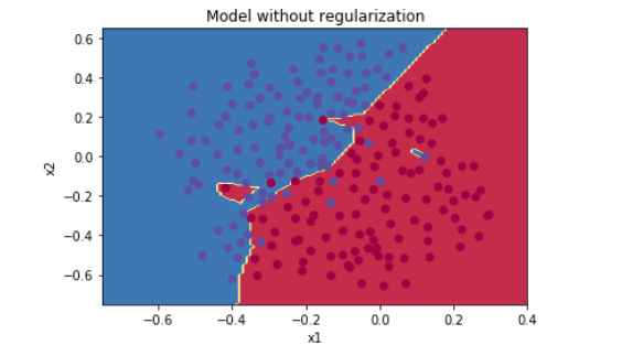
非正则化模型明显是对训练集过拟合，它是对有噪点的拟合!现在让我们看看减少过拟合的两种技术。

2 - L2 Regularization L2正则化

避免过拟合的标准方法称为L2正则化。它包括适当修改你的成本函数，从原来的成本函数(1)到现在的函数(2)：

让我们修改你的成本并观察其结果。

练习：使用正则化()来执行compute_cost_with_regularization()，计算公式(2)所给出的成本。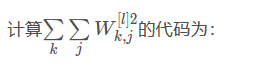　　

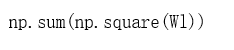
注意，你必须对w[1]， w[2]和w[3]这样做，然后把这三项加起来，再乘以

 1 # GRADED FUNCTION: compute_cost_with_regularization
 2 
 3 def compute_cost_with_regularization(A3, Y, parameters, lambd):
 4     """
 5     Implement the cost function with L2 regularization. 实现公式2的L2正则化计算成本 See formula (2) above.见上式（2）
 6     
 7     Arguments 参数:
 8     A3 -- post-activation, output of forward propagation, of shape (output size, number of examples)激活后，正向传播的输出结果，维度为（输出节点数量，训练/测试的数量）
 9     Y -- "true" labels vector, of shape (output size, number of examples) 标签向量，与数据一一对应，维度为(输出节点数量，训练/测试的数量)
10     parameters -- python dictionary containing parameters of the model 包含模型学习后的参数的字典
11     
12     Returns:
13     cost - value of the regularized loss function (formula (2))使用公式2计算出来的正则化损失的值
14     """
15     m = Y.shape[1]
16     W1 = parameters["W1"]
17     W2 = parameters["W2"]
18     W3 = parameters["W3"]
19     
20     cross_entropy_cost = compute_cost(A3, Y) # This gives you the cross-entropy part of the cost 这就给出了代价的交叉熵部分
21     
22     ### START CODE HERE ### (approx. 1 line)
23     L2_regularization_cost = (1 / m * lambd / 2 )* (np.sum(np.square(W1)) + np.sum(np.square(W2)) + np.sum(np.square(W3)))
24     ### END CODER HERE ###
25     
26     cost = cross_entropy_cost + L2_regularization_cost
27     
28     return cost

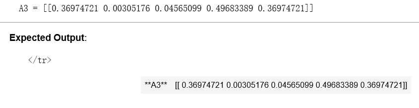
# GRADED FUNCTION: compute_cost_with_regularization

A3, Y_assess, parameters = compute_cost_with_regularization_test_case()

print("cost = " + str(compute_cost_with_regularization(A3, Y_assess, parameters, lambd = 0.1)))

结果：

当然，因为更改了成本，所以也必须更改反向传播!所有的梯度都要根据这个新成本计算。

练习：实现向后传播所需的更改，以考虑正则化。这些更改只涉及dW1、dW2和dW3。对于每一个，你必须加上正则项的梯度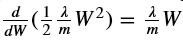

 1 # GRADED FUNCTION: backward_propagation_with_regularization
 2 
 3 def backward_propagation_with_regularization(X, Y, cache, lambd):
 4     """
 5     Implements the backward propagation of our baseline model to which we added an L2 regularization.
 6     
 7     Arguments:
 8     X -- input dataset, of shape (input size, number of examples)输入数据集，维度为（输入节点数量，数据集里面的数量）
 9     Y -- "true" labels vector, of shape (output size, number of examples)标签，维度为（输出节点数量，数据集里面的数量）
10     cache -- cache output from forward_propagation()来自forward_propagation（）的cache输出
11     lambd -- regularization hyperparameter, scalarregularization超参数，实数
12     
13     Returns:
14     gradients -- A dictionary with the gradients with respect to each parameter, activation and pre-activation variables 一个包含了每个参数、激活值和预激活值变量的梯度的字典
15     """
16     
17     m = X.shape[1]
18     (Z1, A1, W1, b1, Z2, A2, W2, b2, Z3, A3, W3, b3) = cache
19     
20     dZ3 = A3 - Y
21     
22     ### START CODE HERE ### (approx. 1 line)
23     dW3 = 1./m * np.dot(dZ3, A2.T) + ((lambd * W3) / m)
24     ### END CODE HERE ###
25     db3 = 1./m * np.sum(dZ3, axis=1, keepdims = True)
26     
27     dA2 = np.dot(W3.T, dZ3)
28     dZ2 = np.multiply(dA2, np.int64(A2 > 0))
29     ### START CODE HERE ### (approx. 1 line)
30     dW2 = 1./m * np.dot(dZ2, A1.T) + ((lambd * W2) / m)
31     ### END CODE HERE ###
32     db2 = 1./m * np.sum(dZ2, axis=1, keepdims = True)
33     
34     dA1 = np.dot(W2.T, dZ2)
35     dZ1 = np.multiply(dA1, np.int64(A1 > 0))
36     ### START CODE HERE ### (approx. 1 line)
37     dW1 = 1./m * np.dot(dZ1, X.T) + ((lambd * W1) / m)
38     ### END CODE HERE ###
39     db1 = 1./m * np.sum(dZ1, axis=1, keepdims = True)
40     
41     gradients = {"dZ3": dZ3, "dW3": dW3, "db3": db3,"dA2": dA2,
42                  "dZ2": dZ2, "dW2": dW2, "db2": db2, "dA1": dA1, 
43                  "dZ1": dZ1, "dW1": dW1, "db1": db1}
44     
45     return gradients

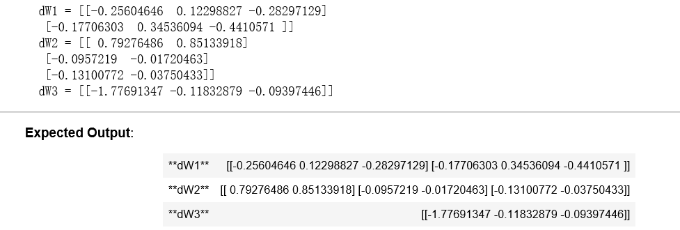
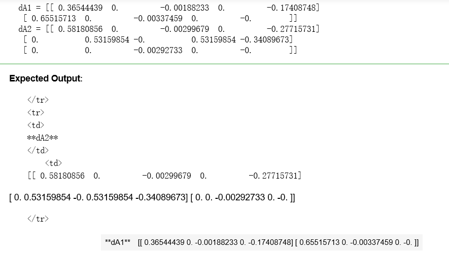
# GRADED FUNCTION: backward_propagation_with_regularization

X_assess, Y_assess, cache = backward_propagation_with_regularization_test_case()

grads = backward_propagation_with_regularization(X_assess, Y_assess, cache, lambd = 0.7)
print ("dW1 = "+ str(grads["dW1"]))
print ("dW2 = "+ str(grads["dW2"]))
print ("dW3 = "+ str(grads["dW3"]))

结果：

现在让我们运行L2正则化的模型。model()函数将调用:

•compute_cost_with_regularization而不是compute_cost
•backward_propagation_with_regularization而不是backward_propagation

parameters = model(train_X, train_Y, lambd = 0.7)
print ("On the train set:")
predictions_train = predict(train_X, train_Y, parameters)
print ("On the test set:")
predictions_test = predict(test_X, test_Y, parameters)

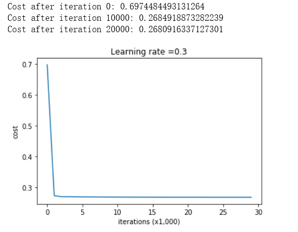
On the train set:

Accuracy: 0.9383886255924171

On the test set:

Accuracy: 0.93

恭喜，测试集的准确率提高到了93%。你救了法国足球队!

你不再过度拟合训练数据了。让我们画出决策边界。

plt.title("Model with L2-regularization")
axes = plt.gca() #Get Current Axes
axes.set_xlim([-0.75,0.40])
axes.set_ylim([-0.75,0.65])
plot_decision_boundary(lambda x: predict_dec(parameters, x.T), train_X, train_Y)

　　python matplotlib.pyplot.gca() 函数的作用（获得当前的Axes对象【Get Current Axes】），参考链接：https://blog.csdn.net/Dontla/article/details/98327176

结果：

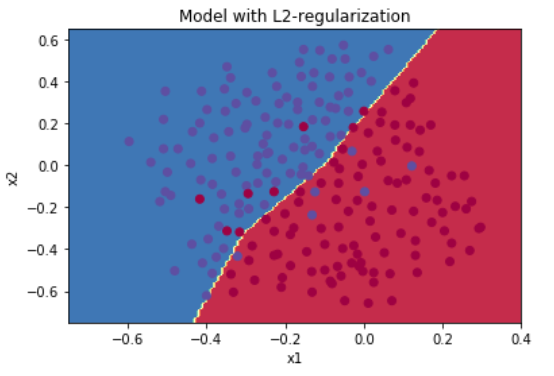
观察：
•您可以使用开发集对其进行优化，其中的值是一个超参数。
•L2正则化使您的决策边界更加平滑。如果拟合太大，也可能会“过度平滑”，导致模型具有高偏差。

l2正规化的实际作用是什么?

l2正则化的前提是，权值较小的模型比权值较大的模型更简单。因此，通过惩罚成本函数中权重的平方值，可以将所有权重都变成更小的值。它变得太昂贵的成本有大的重量!这将产生一个更平滑的模型，在这个模型中，输出随着输入的变化而变化得更慢。

（L2正则化依赖于较小权重的模型比具有较大权重的模型更简单这样的假设，因此，通过削减成本函数中权重的平方值，可以将所有权重值逐渐改变到到较小的值。权值数值高的话会有更平滑的模型，其中输入变化时输出变化更慢，但是你需要花费更多的时间。）

* *你应该记得* *

——L2-regularization的含义:

成本计算：——正则化的计算项需要添加到成本函数中

反向传播功能：——有额外的术语在梯度对权重矩阵,（在权重矩阵方面，梯度计算时也要依据正则化来做出相应的计算）

最终权重变小(“重量衰减”)：——重量推到更小的值。（权重被逐渐改变到较小的值。）

3 - Dropout 随机删除节点

最后，dropout是一种广泛使用的正则化技术，专门用于深度学习。它在每次迭代中随机关闭一些神经元。看看这两个视频，看看这意味着什么!

Figure 2 : Drop-out on the second hidden layer. 图2 第二层启用随机节点删除。

在每次迭代，你关闭(设置为零)一层的每个神经元，概率为1 - keep_prob，我们在这保持它的概率为keep_prob(这里是50%)。在迭代的前向和后向传播中，缺失的神经元对训练都没有贡献。

Figure 3 : Drop-out on the first and third hidden layers. 图3 在第一层和第三层启用随机删除.

第一层:我们平均关闭40%的神经元。第三层:我们平均关闭20%的神经元。

当你关闭一些神经元时，你实际上修改了你的模型。drop-out背后的想法是，在每次迭代中，你训练一个不同的模型，它只使用你神经元的一个子集。有了dropout，你的神经元因此变得对另一个特定神经元的激活不那么敏感，因为另一个神经元可能在任何时候关闭。

3.1 - Forward propagation with dropout 带有dropout的正向传播

练习：使用dropout实现转发。您使用了一个3层的神经网络，并将dropout添加到第一层和第二层隐藏层。我们不会将dropout应用到输入层或输出层。

说明：你想关闭第一层和第二层的一些神经元。要做到这一点，你需要执行4个步骤：

1.在讲座中，我们讨论了使用np.random.rand()创建一个与a^[1]具有相同形状的变量d^[1]，以随机获取0到1之间的数字。这里，您将使用向量化实现，因此创建一个随机矩阵D^[1] =[D ^[1]₍₁₎ D^[1]₍₂₎…与A^[1]维数相同的。

2.通过适当地对D^[1]中的值进行阈值设定，将D^[1]的每个条目的概率设为0 (1-keep_prob)或概率设为1 (keep_prob)。提示:要将矩阵X的所有项设为0(如果项小于0.5)或1(如果项大于0.5)，您可以这样做：X = (X < 0.5)。注意，0和1分别等同于False和True。

3.将A[1]设置为A^[1]∗D^[1]。(你正在关闭一些神经元)。你可以把d^[1]看作一个掩码，当它与另一个矩阵相乘时，它会关闭一些值。

4.A^[1]除以keep_prob。通过这样做，您可以确保成本的结果仍然具有与没有dropout相同的期望值。(这种技术也被称为反向dropout。)

 1 # GRADED FUNCTION: forward_propagation_with_dropout
 2 
 3 def forward_propagation_with_dropout(X, parameters, keep_prob = 0.5):
 4     """
 5     Implements the forward propagation: LINEAR -> RELU + DROPOUT -> LINEAR -> RELU + DROPOUT -> LINEAR -> SIGMOID.
 6     实现具有随机舍弃节点的前向传播。
 7     Arguments:
 8     X -- input dataset, of shape (2, number of examples)
 9     parameters -- python dictionary containing your parameters "W1", "b1", "W2", "b2", "W3", "b3":
10                     W1 -- weight matrix of shape (20, 2)
11                     b1 -- bias vector of shape (20, 1) 偏向量
12                     W2 -- weight matrix of shape (3, 20)
13                     b2 -- bias vector of shape (3, 1)
14                     W3 -- weight matrix of shape (1, 3)
15                     b3 -- bias vector of shape (1, 1)
16     keep_prob - probability of keeping a neuron active during drop-out, scalar 随机删除的概率，实数
17     
18     Returns:
19     A3 -- last activation value, output of the forward propagation, of shape (1,1) 最后的激活值，维度为（1,1），正向传播的输出
20     cache -- tuple, information stored for computing the backward propagation  存储了一些用于计算反向传播的数值的元组
21     """
22     
23     np.random.seed(1)
24     
25     # retrieve parameters
26     W1 = parameters["W1"]
27     b1 = parameters["b1"]
28     W2 = parameters["W2"]
29     b2 = parameters["b2"]
30     W3 = parameters["W3"]
31     b3 = parameters["b3"]
32     
33     # LINEAR -> RELU -> LINEAR -> RELU -> LINEAR -> SIGMOID
34     Z1 = np.dot(W1, X) + b1
35     A1 = relu(Z1)
36     ### START CODE HERE ### (approx. 4 lines)         # Steps 1-4 below correspond to the Steps 1-4 described above. 下面的步骤1-4对应于上述的步骤1-4。
37     D1 = np.random.rand(A1.shape[0], A1.shape[1])     # Step 1: initialize matrix D1 = np.random.rand(..., ...) 初始化矩阵D1 = np.random.rand(..., ...)
38     D1 = D1<keep_prob                                 # Step 2: convert entries of D1 to 0 or 1 (using keep_prob as the threshold)将D1的值转换为0或1（使用keep_prob作为阈值）
39     A1 = A1 * D1                                      # Step 3: shut down some neurons of A1 的一些节点（将它的值变为0或False）
40     A1 = A1 / keep_prob                               # Step 4: scale the value of neurons that haven't been shut down 缩放未舍弃的节点(不为0)的值
41     ### END CODE HERE ###
42     Z2 = np.dot(W2, A1) + b2
43     A2 = relu(Z2)
44     ### START CODE HERE ### (approx. 4 lines)
45     D2 = np.random.rand(A2.shape[0], A2.shape[1])      # Step 1: initialize matrix D2 = np.random.rand(..., ...) 初始化矩阵D2 = np.random.rand(..., ...)
46     D2 = D2 < keep_prob                                # Step 2: convert entries of D2 to 0 or 1 (using keep_prob as the threshold) 将D2的值转换为0或1（使用keep_prob作为阈值）
47     A2 = A2 * D2                                       # Step 3: shut down some neurons of A2 舍弃A1的一些节点（将它的值变为0或False） 舍弃A1的一些节点（将它的值变为0或False）
48     A2 = A2 / keep_prob                                # Step 4: scale the value of neurons that haven't been shut down 缩放未舍弃的节点(不为0)的值
49     ### END CODE HERE ###
50     Z3 = np.dot(W3, A2) + b3
51     A3 = sigmoid(Z3)
52     
53     cache = (Z1, D1, A1, W1, b1, Z2, D2, A2, W2, b2, Z3, A3, W3, b3)
54     
55     return A3, cache

# GRADED FUNCTION: forward_propagation_with_dropout

X_assess, parameters = forward_propagation_with_dropout_test_case()

A3, cache = forward_propagation_with_dropout(X_assess, parameters, keep_prob = 0.7)
print ("A3 = " + str(A3))

3.2 - Backward propagation with dropout 使用dropout的反向传播

练习：使用dropout实现向后传播。与前面一样，您正在训练一个3层网络。使用存储在缓存中的掩码D^[1]和D^[2]，在第一和第二隐藏层添加dropout。

说明:带dropout的反向传播实际上很容易。您将必须执行两个步骤：

1.在前向传播的过程中，通过对A1施加一个掩码D^[1]，你已经关闭了一些神经元。在反向传播中，你必须通过对dA1重新应用相同的掩码D^[1]来关闭相同的神经元。

2.在前向传播期间，您将A1除以keep_prob。在反向传播中，您将不得不再次将dA1除以keep_prob(微积分解释是，如果一个A^[1]被keep_prob缩放，那么它的导数dA^[1]也被相同的keep_prob缩放)。

# GRADED FUNCTION: backward_propagation_with_dropout

def backward_propagation_with_dropout(X, Y, cache, keep_prob):
    """
    Implements the backward propagation of our baseline model to which we added dropout.
    
    Arguments:
    X -- input dataset, of shape (2, number of examples)
    Y -- "true" labels vector, of shape (output size, number of examples)
    cache -- cache output from forward_propagation_with_dropout() 来自forward_propagation_with_dropout（）的cache输出
    keep_prob - probability of keeping a neuron active during drop-out, scalar 随机删除的概率，实数
    
    Returns:
    gradients -- A dictionary with the gradients with respect to each parameter, activation and pre-activation variables 一个关于每个参数、激活值和预激活变量的梯度值的字典
    """
    
    m = X.shape[1]
    (Z1, D1, A1, W1, b1, Z2, D2, A2, W2, b2, Z3, A3, W3, b3) = cache
    
    dZ3 = A3 - Y
    dW3 = 1./m * np.dot(dZ3, A2.T)
    db3 = 1./m * np.sum(dZ3, axis=1, keepdims = True)
    dA2 = np.dot(W3.T, dZ3)
    ### START CODE HERE ### (≈ 2 lines of code)
    dA2 = dA2 * D2              # Step 1: Apply mask D2 to shut down the same neurons as during the forward propagation使用正向传播期间相同的节点，舍弃那些关闭的节点（因为任何数乘以0或者False都为0或者False）
    dA2 = dA2 / keep_prob              # Step 2: Scale the value of neurons that haven't been shut down 缩放未舍弃的节点(不为0)的值
    ### END CODE HERE ###
    dZ2 = np.multiply(dA2, np.int64(A2 > 0))
    dW2 = 1./m * np.dot(dZ2, A1.T)
    db2 = 1./m * np.sum(dZ2, axis=1, keepdims = True)
    
    dA1 = np.dot(W2.T, dZ2)
    ### START CODE HERE ### (≈ 2 lines of code)
    dA1 = dA1 * D1              # Step 1: Apply mask D1 to shut down the same neurons as during the forward propagation 使用正向传播期间相同的节点，舍弃那些关闭的节点（因为任何数乘以0或者False都为0或者False）
    dA1 = dA1 / keep_prob              # Step 2: Scale the value of neurons that haven't been shut down 缩放未舍弃的节点(不为0)的值
    ### END CODE HERE ###
    dZ1 = np.multiply(dA1, np.int64(A1 > 0))
    dW1 = 1./m * np.dot(dZ1, X.T)
    db1 = 1./m * np.sum(dZ1, axis=1, keepdims = True)
    
    gradients = {"dZ3": dZ3, "dW3": dW3, "db3": db3,"dA2": dA2,
                 "dZ2": dZ2, "dW2": dW2, "db2": db2, "dA1": dA1, 
                 "dZ1": dZ1, "dW1": dW1, "db1": db1}
    
    return gradients

X_assess, Y_assess, cache = backward_propagation_with_dropout_test_case()

gradients = backward_propagation_with_dropout(X_assess, Y_assess, cache, keep_prob = 0.8)

print ("dA1 = " + str(gradients["dA1"]))
print ("dA2 = " + str(gradients["dA2"]))

结果：

现在让我们运行带有dropout (keep_prob = 0.86)的模型。这意味着在每次迭代中，以24%的概率关闭第1层和第2层的每个神经元。函数model()现在将调用：
•forward_propagation_with_dropout而不是forward_propagation。
•backward_propagation_with_dropout而不是backward_propagation。

parameters = model(train_X, train_Y, keep_prob = 0.86, learning_rate = 0.3)

print ("On the train set:")
predictions_train = predict(train_X, train_Y, parameters)
print ("On the test set:")
predictions_test = predict(test_X, test_Y, parameters)

结果：

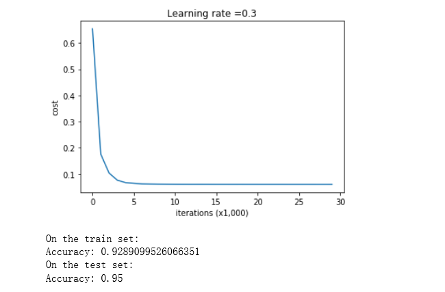
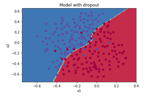
dropout干的很好!测试准确度再次提高(到95%)!你的模型没有过度拟合训练集，而且在测试集上做得很好。法国足球队将永远感谢你!

运行下面的代码来绘制决策边界。

plt.title("Model with dropout")
axes = plt.gca()
axes.set_xlim([-0.75,0.40])
axes.set_ylim([-0.75,0.65])
plot_decision_boundary(lambda x: predict_dec(parameters, x.T), train_X, train_Y)

注意：
•在使用dropout时，一个常见的错误是在训练和测试中都使用它。您应该只在训练中使用dropout(随机删除节点)。
•深度学习框架，如tensorflow, PaddlePaddle, keras或caffe都带有dropout层实现。不要紧张——你很快就会学到其中一些框架。
关于dropout你应该记住的是:**

- dropout是一种正则化技术。

-你只在训练期间使用dropout。在测试期间不要使用dropout(随机删除节点)。

-在正向传播和反向传播期间应用dropout。

-在训练期间，用keep_prob对每个dropout层进行划分，以保持激活的期望值相同。例如，如果keep_prob是0.5，那么我们将平均关闭一半节点，因此输出将按0.5进行缩放，因为只有剩下的一半对解决方案有贡献。除以0.5等于乘以2。因此，输出现在具有相同的期望值。您可以检查，即使在keep_prob的值不是0.5时，这个方法也可以工作。

4 - Conclusions 结论

以下是我们三个模型的结果:

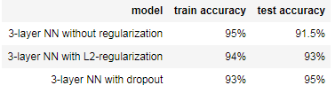
注意，正则化会影响训练集的性能!这是因为它限制了网络过度适应训练集的能力。但由于它最终提供了更好的测试准确性，它有助于您的系统。

恭喜你完成了这项任务!以及法国足球的革命。:-)

**我们希望你从这个笔记本中记住的东西**:

-正则化将帮助你减少过拟合。

-正规化将使你的权重值降低。

- L2正则化和Dropout正则化是两种非常有效的正则化技术。

posted @ 2020-07-29 16:11 廖海清阅读(1452) 评论(0) 编辑收藏举报

会员力量，点亮园子希望

刷新页面返回顶部

Agiroy_70's Blog

吴恩达深度学习第二课第一周编程作业_regularization（正则化）

Regularization 正则化

声明

1 - Non-regularized model 无正则化的模型

2 - L2 Regularization L2正则化

3 - Dropout 随机删除节点

3.1 - Forward propagation with dropout 带有dropout的正向传播

3.2 - Backward propagation with dropout 使用dropout的反向传播

4 - Conclusions 结论

公告

Agiroy_70's Blog

吴恩达深度学习 第二课第一周编程作业_regularization（正则化）

Regularization 正则化

声明

1 - Non-regularized model 无正则化的模型

2 - L2 Regularization L2正则化

3 - Dropout 随机删除节点

3.1 - Forward propagation with dropout 带有dropout的正向传播

3.2 - Backward propagation with dropout 使用dropout的反向传播

4 - Conclusions 结论

公告

吴恩达深度学习第二课第一周编程作业_regularization（正则化）