卷积神经网络的直观解释

本文章翻译自the data science blog中的《An Intuitive Explanation of Convolutional Neural Networks》

作者：ujjwalkarn
原文日期：2016 年 8 月 11 日

1. 什么是卷积神经网络？为什么它们很重要？

卷积神经网络（ConvNets 或者 CNNs）属于神经网络的范畴，已经在诸如图像识别和分类的领域证明了其高效的能力。卷积神经网络可以成功识别人脸、物体和交通信号，从而为机器人和自动驾驶汽车提供视力。

在图1中，卷积神经网络可以识别场景，也可以提供相关的标签，比如“桥梁”、“火车”和“网球”；而下图展示了卷积神经网络可以用来识别日常物体、人和动物。最近，卷积神经网络也在一些自然语言处理任务（比如语句分类）上面展示了良好的效果。

因此，卷积神经网络对于今天大多数的机器学习用户来说都是一个重要的工具。然而，理解卷积神经网络以及首次学习使用它们有时会很痛苦。那本篇博客的主要目的就是让我们对卷积神经网络如何处理图像有一个基本的了解。

如果你是神经网络的新手，我建议你阅读下这篇短小的多层感知器的教程，在进一步阅读前对神经网络有一定的理解。在本篇博客中，多层感知器叫做“全连接层”。

2. LeNet架构(1990s)

LeNet 是推进深度学习领域发展的最早的卷积神经网络之一。经过多次成功迭代，到 1988 年，Yann LeCun 把这一先驱工作命名为 LeNet5。当时，LeNet 架构主要用于字符识别任务，比如读取邮政编码、数字等等。

接下来，我们将会了解 LeNet 架构是如何学会识别图像的。近年来有许多在 LeNet 上面改进的新架构被提出来，但它们都使用了 LeNet 中的主要概念，如果你对 LeNet 有一个清晰的认识，就相对比较容易理解。

图3中的卷积神经网络和原始的 LeNet 的结构比较相似，可以把输入的图像分为四类：狗、猫、船或者鸟（原始的 LeNet 主要用于字符识别任务）。正如上图说示，当输入为一张船的图片时，网络可以正确的从四个类别中把最高的概率分配给船（0.94）。在输出层所有概率的和应该为一（本文稍后会解释）。

在图3中ConvNet有四个主要操作：

1.卷积
2.非线性处理(ReLU)
3.池化(亚采样)
4.分类(全连接层)

这些操作对于各个卷积神经网络来说都是基本组件，因此理解它们的工作原理有助于充分了解卷积神经网络。下面我们将会尝试理解各步操作背后的原理。

3. 图像时像素值的矩阵

本质上来说，每张图像都可以表示为像素值的矩阵：

Figure 4: Every image is a matrix of pixel values. Source [6]

通道 常用于表示图像的某种组成。一个标准数字相机拍摄的图像会有三通道 - 红、绿和蓝；你可以把它们看作是互相堆叠在一起的二维矩阵（每一个通道代表一个颜色），每个通道的像素值在 0 到 255 的范围内。

灰度图像，仅仅只有一个通道。在本篇文章中，我们仅考虑灰度图像，这样我们就只有一个二维的矩阵来表示图像。矩阵中各个像素的值在 0 到 255 的范围内——零表示黑色，255 表示白色。

4. 卷积的步骤

卷积神经网络的名字就来自于其中的卷积操作。卷积的主要目的是为了从输入图像中提取特征。卷积可以通过从输入的一小块数据中学到图像的特征，并可以保留像素间的空间关系。我们在这里并不会详细讲解卷积的数学细节，但我们会试着理解卷积是如何处理图像的。

正如我们上面所说，每张图像都可以看作是像素值的矩阵。考虑一下一个 5 x 5 的图像，它的像素值仅为 0 或者 1（注意对于灰度图像而言，像素值的范围是 0 到 255，下面像素值为 0 和 1 的绿色矩阵仅为特例）：

同时，考虑下另一个 3 x 3 的矩阵，如下所示：

接下来，5 x 5 的图像和 3 x 3 的矩阵的卷积可以按下图所示的动画一样计算：

Figure 5: The Convolution operation. The output matrix is called Convolved Feature or Feature Map. Source [7]

现在停下来好好理解下上面的计算是怎么完成的。我们用橙色的矩阵在原始图像（绿色）上滑动，每次滑动一个像素（也叫做“步长”），在每个位置上，我们计算对应元素的乘积（两个矩阵间），并把乘积的和作为最后的结果，得到输出矩阵（粉色）中的每一个元素的值。注意，3 x 3 的矩阵每次步长中仅可以“看到”输入图像的一部分。

在 CNN 的术语中，3x3 的矩阵叫做“滤波器（filter）”或者“核（kernel）”或者“特征检测器（feature detector）”，通过在图像上滑动滤波器并计算点乘得到矩阵叫做“卷积特征（Convolved Feature）”或者“激活图（Activation Map）”或者“特征图（Feature Map）”。记住滤波器在原始输入图像上的作用是特征检测器。

It is evident from the animation above that different values of the filter matrix will produce different Feature Maps for the same input image. As an example, consider the following input image:

从上面图中的动画可以看出，对于同样的输入图像，不同值的滤波器将会生成不同的特征图。比如，对于下面这张输入图像：

In the table below, we can see the effects of convolution of the above image with different filters. As shown, we can perform operations such as Edge Detection, Sharpen and Blur just by changing the numeric values of our filter matrix before the convolution operation [8] – this means that different filters can detect different features from an image, for example edges, curves etc. More such examples are available in Section 8.2.4 here.

Another good way to understand the Convolution operation is by looking at the animation in Figure 6 below:

Figure 6: The Convolution Operation. Source [9]

A filter (with red outline) slides over the input image (convolution operation) to produce a feature map. The convolution of another filter (with the green outline), over the same image gives a different feature map as shown. It is important to note that the Convolution operation captures the local dependencies in the original image. Also notice how these two different filters generate different feature maps from the same original image. Remember that the image and the two filters above are just numeric matrices as we have discussed above.

In practice, a CNN learns the values of these filters on its own during the training process (although we still need to specify parameters such as number of filters, filter size, architecture of the networketc. before the training process). The more number of filters we have, the more image features get extracted and the better our network becomes at recognizing patterns in unseen images.

The size of the Feature Map (Convolved Feature) is controlled by three parameters [4] that we need to decide before the convolution step is performed:

• Depth: Depth corresponds to the number of filters we use for the convolution operation. In the network shown in Figure 7, we are performing convolution of the original boat image using three distinct filters, thus producing three different feature maps as shown. You can think of these three feature maps as stacked 2d matrices, so, the ‘depth’ of the feature map would be three.

Figure 7

• Stride: Stride is the number of pixels by which we slide our filter matrix over the input matrix. When the stride is 1 then we move the filters one pixel at a time. When the stride is 2, then the filters jump 2 pixels at a time as we slide them around. Having a larger stride will produce smaller feature maps.

• Zero-padding: Sometimes, it is convenient to pad the input matrix with zeros around the border, so that we can apply the filter to bordering elements of our input image matrix. A nice feature of zero padding is that it allows us to control the size of the feature maps. Adding zero-padding is also called wide convolution, and not using zero-padding would be a narrow convolution. This has been explained clearly in [14].

Introducing Non Linearity (ReLU)

An additional operation called ReLU has been used after every Convolution operation in Figure 3 above. ReLU stands for Rectified Linear Unit and is a non-linear operation. Its output is given by:

Figure 8: the ReLU operation

ReLU is an element wise operation (applied per pixel) and replaces all negative pixel values in the feature map by zero. The purpose of ReLU is to introduce non-linearity in our ConvNet, since most of the real-world data we would want our ConvNet to learn would be non-linear (Convolution is a linear operation – element wise matrix multiplication and addition, so we account for non-linearity by introducing a non-linear function like ReLU).

The ReLU operation can be understood clearly from Figure 9 below. It shows the ReLU operation applied to one of the feature maps obtained in Figure 6 above. The output feature map here is also referred to as the ‘Rectified’ feature map.

Figure 9: ReLU operation. Source [10]

Other non linear functions such as tanh or sigmoid can also be used instead of ReLU, but ReLU has been found to perform better in most situations.

The Pooling Step

Spatial Pooling (also called subsampling or downsampling) reduces the dimensionality of each feature map but retains the most important information. Spatial Pooling can be of different types: Max, Average, Sum etc.

In case of Max Pooling, we define a spatial neighborhood (for example, a 2×2 window) and take the largest element from the rectified feature map within that window. Instead of taking the largest element we could also take the average (Average Pooling) or sum of all elements in that window. In practice, Max Pooling has been shown to work better.

Figure 10 shows an example of Max Pooling operation on a Rectified Feature map (obtained after convolution + ReLU operation) by using a 2×2 window.

Figure 10: Max Pooling. Source [4]

We slide our 2 x 2 window by 2 cells (also called ‘stride’) and take the maximum value in each region. As shown in Figure 10, this reduces the dimensionality of our feature map.

In the network shown in Figure 11, pooling operation is applied separately to each feature map (notice that, due to this, we get three output maps from three input maps).

Figure 11: Pooling applied to Rectified Feature Maps

Figure 12 shows the effect of Pooling on the Rectified Feature Map we received after the ReLU operation in Figure 9 above.

Figure 12: Pooling. Source [10]

The function of Pooling is to progressively reduce the spatial size of the input representation [4]. In particular, pooling

• makes the input representations (feature dimension) smaller and more manageable
• reduces the number of parameters and computations in the network, therefore, controlling overfitting [4]
• makes the network invariant to small transformations, distortions and translations in the input image (a small distortion in input will not change the output of Pooling – since we take the maximum / average value in a local neighborhood).
• helps us arrive at an almost scale invariant representation of our image (the exact term is “equivariant”). This is very powerful since we can detect objects in an image no matter where they are located (read [18] and [19] for details).

Story so far

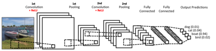
Figure 13

So far we have seen how Convolution, ReLU and Pooling work. It is important to understand that these layers are the basic building blocks of any CNN. As shown in Figure 13, we have two sets of Convolution, ReLU & Pooling layers – the 2nd Convolution layer performs convolution on the output of the first Pooling Layer using six filters to produce a total of six feature maps. ReLU is then applied individually on all of these six feature maps. We then perform Max Pooling operation separately on each of the six rectified feature maps.

Together these layers extract the useful features from the images, introduce non-linearity in our network and reduce feature dimension while aiming to make the features somewhat equivariant to scale and translation [18].

The output of the 2nd Pooling Layer acts as an input to the Fully Connected Layer, which we will discuss in the next section.

Fully Connected Layer

The Fully Connected layer is a traditional Multi Layer Perceptron that uses a softmax activation function in the output layer (other classifiers like SVM can also be used, but will stick to softmax in this post). The term “Fully Connected” implies that every neuron in the previous layer is connected to every neuron on the next layer. I recommend reading this post if you are unfamiliar with Multi Layer Perceptrons.

The output from the convolutional and pooling layers represent high-level features of the input image. The purpose of the Fully Connected layer is to use these features for classifying the input image into various classes based on the training dataset. For example, the image classification task we set out to perform has four possible outputs as shown in Figure 14 below (note that Figure 14 does not show connections between the nodes in the fully connected layer)

Figure 14: Fully Connected Layer -each node is connected to every other node in the adjacent layer

Apart from classification, adding a fully-connected layer is also a (usually) cheap way of learning non-linear combinations of these features. Most of the features from convolutional and pooling layers may be good for the classification task, but combinations of those features might be even better [11].

The sum of output probabilities from the Fully Connected Layer is 1. This is ensured by using the Softmax as the activation function in the output layer of the Fully Connected Layer. The Softmax function takes a vector of arbitrary real-valued scores and squashes it to a vector of values between zero and one that sum to one.

Putting it all together – Training using Backpropagation

As discussed above, the Convolution + Pooling layers act as Feature Extractors from the input image while Fully Connected layer acts as a classifier.

Note that in Figure 15 below, since the input image is a boat, the target probability is 1 for Boat class and 0 for other three classes, i.e.

• Input Image = Boat
• Target Vector = [0, 0, 1, 0]

Figure 15: Training the ConvNet

The overall training process of the Convolution Network may be summarized as below:

• Step1: We initialize all filters and parameters / weights with random values

• Step2:

  The network takes a training image as input, goes through the forward propagation step (convolution, ReLU and pooling operations along with forward propagation in the Fully Connected layer) and finds the output probabilities for each class.

  • Lets say the output probabilities for the boat image above are [0.2, 0.4, 0.1, 0.3]
  • Since weights are randomly assigned for the first training example, output probabilities are also random.

• Step3:

  Calculate the total error at the output layer (summation over all 4 classes)

  • Total Error = ∑ ½ (target probability – output probability) ²

• Step4:

  Use Backpropagation to calculate the

  gradients

  of the error with respect to all weights in the network and use

  gradient descent

  to update all filter values / weights and parameter values to minimize the output error.

  • The weights are adjusted in proportion to their contribution to the total error.
  • When the same image is input again, output probabilities might now be [0.1, 0.1, 0.7, 0.1], which is closer to the target vector [0, 0, 1, 0].
  • This means that the network has learnt to classify this particular image correctly by adjusting its weights / filters such that the output error is reduced.
  • Parameters like number of filters, filter sizes, architecture of the network etc. have all been fixed before Step 1 and do not change during training process – only the values of the filter matrix and connection weights get updated.

• Step5: Repeat steps 2-4 with all images in the training set.

The above steps train the ConvNet – this essentially means that all the weights and parameters of the ConvNet have now been optimized to correctly classify images from the training set.

When a new (unseen) image is input into the ConvNet, the network would go through the forward propagation step and output a probability for each class (for a new image, the output probabilities are calculated using the weights which have been optimized to correctly classify all the previous training examples). If our training set is large enough, the network will (hopefully) generalize well to new images and classify them into correct categories.

Note 1: The steps above have been oversimplified and mathematical details have been avoided to provide intuition into the training process. See [4] and [12] for a mathematical formulation and thorough understanding.

Note 2: In the example above we used two sets of alternating Convolution and Pooling layers. Please note however, that these operations can be repeated any number of times in a single ConvNet. In fact, some of the best performing ConvNets today have tens of Convolution and Pooling layers! Also, it is not necessary to have a Pooling layer after every Convolutional Layer. As can be seen in the Figure 16 below, we can have multiple Convolution + ReLU operations in succession before having a Pooling operation. Also notice how each layer of the ConvNet is visualized in the Figure 16 below.

Figure 16: Source [4]

Visualizing Convolutional Neural Networks

In general, the more convolution steps we have, the more complicated features our network will be able to learn to recognize. For example, in Image Classification a ConvNet may learn to detect edges from raw pixels in the first layer, then use the edges to detect simple shapes in the second layer, and then use these shapes to deter higher-level features, such as facial shapes in higher layers [14]. This is demonstrated in Figure 17 below – these features were learnt using a Convolutional Deep Belief Network and the figure is included here just for demonstrating the idea (this is only an example: real life convolution filters may detect objects that have no meaning to humans).

Figure 17: Learned features from a Convolutional Deep Belief Network. Source [21]

Adam Harley created amazing visualizations of a Convolutional Neural Network trained on the MNIST Database of handwritten digits [13]. I highly recommend playing around with it to understand details of how a CNN works.

We will see below how the network works for an input ‘8’. Note that the visualization in Figure 18does not show the ReLU operation separately.

Figure 18: Visualizing a ConvNet trained on handwritten digits. Source [13]

The input image contains 1024 pixels (32 x 32 image) and the first Convolution layer (Convolution Layer 1) is formed by convolution of six unique 5 × 5 (stride 1) filters with the input image. As seen, using six different filters produces a feature map of depth six.

Convolutional Layer 1 is followed by Pooling Layer 1 that does 2 × 2 max pooling (with stride 2) separately over the six feature maps in Convolution Layer 1. You can move your mouse pointer over any pixel in the Pooling Layer and observe the 2 x 2 grid it forms in the previous Convolution Layer (demonstrated in Figure 19). You’ll notice that the pixel having the maximum value (the brightest one) in the 2 x 2 grid makes it to the Pooling layer.

Figure 19: Visualizing the Pooling Operation. Source [13]

Pooling Layer 1 is followed by sixteen 5 × 5 (stride 1) convolutional filters that perform the convolution operation. This is followed by Pooling Layer 2 that does 2 × 2 max pooling (with stride 2). These two layers use the same concepts as described above.

We then have three fully-connected (FC) layers. There are:

• 120 neurons in the first FC layer
• 100 neurons in the second FC layer
• 10 neurons in the third FC layer corresponding to the 10 digits – also called the Output layer

Notice how in Figure 20, each of the 10 nodes in the output layer are connected to all 100 nodes in the 2nd Fully Connected layer (hence the name Fully Connected).

Also, note how the only bright node in the Output Layer corresponds to ‘8’ – this means that the network correctly classifies our handwritten digit (brighter node denotes that the output from it is higher, i.e. 8 has the highest probability among all other digits).

Figure 20: Visualizing the Filly Connected Layers. Source [13]

The 3d version of the same visualization is available here.

Other ConvNet Architectures

Convolutional Neural Networks have been around since early 1990s. We discussed the LeNet above which was one of the very first convolutional neural networks. Some other influential architectures are listed below [3] [4].

• LeNet (1990s): Already covered in this article.

• 1990s to 2012: In the years from late 1990s to early 2010s convolutional neural network were in incubation. As more and more data and computing power became available, tasks that convolutional neural networks could tackle became more and more interesting.

• AlexNet (2012) – In 2012, Alex Krizhevsky (and others) released AlexNet which was a deeper and much wider version of the LeNet and won by a large margin the difficult ImageNet Large Scale Visual Recognition Challenge (ILSVRC) in 2012. It was a significant breakthrough with respect to the previous approaches and the current widespread application of CNNs can be attributed to this work.

• ZF Net (2013) – The ILSVRC 2013 winner was a Convolutional Network from Matthew Zeiler and Rob Fergus. It became known as the ZFNet (short for Zeiler & Fergus Net). It was an improvement on AlexNet by tweaking the architecture hyperparameters.

• GoogLeNet (2014) – The ILSVRC 2014 winner was a Convolutional Network from Szegedy et al.from Google. Its main contribution was the development of an Inception Module that dramatically reduced the number of parameters in the network (4M, compared to AlexNet with 60M).

• VGGNet (2014) – The runner-up in ILSVRC 2014 was the network that became known as the VGGNet. Its main contribution was in showing that the depth of the network (number of layers) is a critical component for good performance.

• ResNets (2015) – Residual Network developed by Kaiming He (and others) was the winner of ILSVRC 2015. ResNets are currently by far state of the art Convolutional Neural Network models and are the default choice for using ConvNets in practice (as of May 2016).

• DenseNet (August 2016) – Recently published by Gao Huang (and others), the Densely Connected Convolutional Network has each layer directly connected to every other layer in a feed-forward fashion. The DenseNet has been shown to obtain significant improvements over previous state-of-the-art architectures on five highly competitive object recognition benchmark tasks. Check out the Torch implementation here.

Conclusion

In this post, I have tried to explain the main concepts behind Convolutional Neural Networks in simple terms. There are several details I have oversimplified / skipped, but hopefully this post gave you some intuition around how they work.

This post was originally inspired from Understanding Convolutional Neural Networks for NLP by Denny Britz (which I would recommend reading) and a number of explanations here are based on that post. For a more thorough understanding of some of these concepts, I would encourage you to go through the notes from Stanford’s course on ConvNets as well as other excellent resources mentioned under References below. If you face any issues understanding any of the above concepts or have questions / suggestions, feel free to leave a comment below.

All images and animations used in this post belong to their respective authors as listed in References section below.

References

1. karpathy/neuraltalk2: Efficient Image Captioning code in Torch, Examples
2. Shaoqing Ren, et al, “Faster R-CNN: Towards Real-Time Object Detection with Region Proposal Networks”, 2015, arXiv:1506.01497
3. Neural Network Architectures, Eugenio Culurciello’s blog
4. CS231n Convolutional Neural Networks for Visual Recognition, Stanford
5. Clarifai / Technology
6. Machine Learning is Fun! Part 3: Deep Learning and Convolutional Neural Networks
7. Feature extraction using convolution, Stanford
8. Wikipedia article on Kernel (image processing)
9. Deep Learning Methods for Vision, CVPR 2012 Tutorial
10. Neural Networks by Rob Fergus, Machine Learning Summer School 2015
11. What do the fully connected layers do in CNNs?
12. Convolutional Neural Networks, Andrew Gibiansky
13. A. W. Harley, “An Interactive Node-Link Visualization of Convolutional Neural Networks,” in ISVC, pages 867-877, 2015 (link). Demo
14. Understanding Convolutional Neural Networks for NLP
15. Backpropagation in Convolutional Neural Networks
16. A Beginner’s Guide To Understanding Convolutional Neural Networks
17. Vincent Dumoulin, et al, “A guide to convolution arithmetic for deep learning”, 2015, arXiv:1603.07285
18. What is the difference between deep learning and usual machine learning?
19. How is a convolutional neural network able to learn invariant features?
20. A Taxonomy of Deep Convolutional Neural Nets for Computer Vision
21. Honglak Lee, et al, “Convolutional Deep Belief Networks for Scalable Unsupervised Learning of Hierarchical Representations” (link)

Share this: