
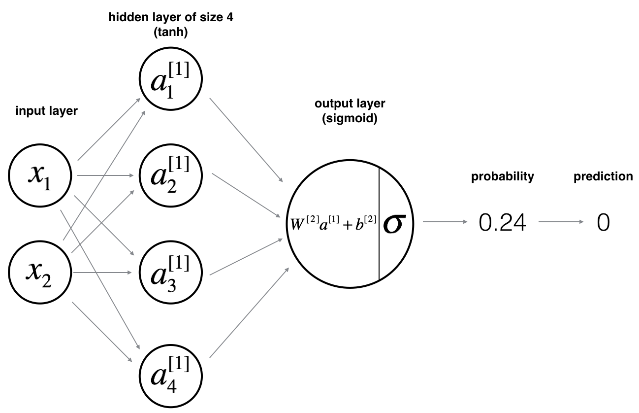
线性与非线性激活函数的作用(以一个2层的神经网络为例)
想起来之前做过的一个吴恩达sir的课后作业,复习了一遍加强理解。
按照前人的经验通常把sigmoid()只用在最后一层上,所以前面的那一层就用relu()。sigmoid层结束其实就算是出结果了
1.导包/库
import numpy as np
import matplotlib.pyplot as plt
from testCases import *
import sklearn
import sklearn.datasets
import sklearn.linear_model
from planar_utils import plot_decision_boundary, sigmoid, load_planar_dataset, load_extra_datasets

%matplotlib inline
2.加载数据
这里用的是网上给的一个方法,正好是一个花的形状,真忘了叫什么花了,之前在花书上看到过,不过没在手边,我查了一下也没查到,算是一个比较经典的比较线性和非线性模型的数据集。
X, Y = load_planar_dataset()
运行下面的代码可以看到花长什么样
plt.scatter(X[0, :], X[1, :], c=Y[0, :], s=40, cmap=plt.cm.Spectral);
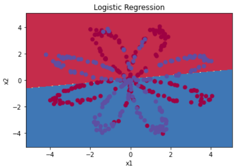
3.先看看线性模型训练出来会是什么样的
clf = sklearn.linear_model.LogisticRegressionCV()
clf.fit(X.T, Y[0, :].T)

def plot_decision_boundary(model, X, y):
    # Set min and max values and give it some padding
    x_min, x_max = X[0, :].min() - 1, X[0, :].max() + 1
    y_min, y_max = X[1, :].min() - 1, X[1, :].max() + 1
    h = 0.01
    # Generate a grid of points with distance h between them
    xx, yy = np.meshgrid(np.arange(x_min, x_max, h), np.arange(y_min, y_max, h))
    # Predict the function value for the whole grid
    Z = model(np.c_[xx.ravel(), yy.ravel()])
    Z = Z.reshape(xx.shape)
    # Plot the contour and training examples
    plt.contourf(xx, yy, Z, cmap=plt.cm.Spectral)
    plt.ylabel('x2')
    plt.xlabel('x1')
    plt.scatter(X[0, :], X[1, :], c=y, cmap=plt.cm.Spectral)

plot_decision_boundary(lambda x: clf.predict(x), X, Y[0, :])
plt.title("Logistic Regression")
可以到的这么一个笨蛋结果,不需要思考就知道这个结果肯定是笨的不谈,接下来手把手再实现一个线性模型。
4.先定义一下要用的模型,主要是每个层的节点数。(不得不说吴恩达sir教我写代码真是可以说是手把手了)
def layer_sizes(X, Y):
    """
    Returns:
    n_x -- the size of the input layer
    n_h -- the size of the hidden layer
    n_y -- the size of the output layer
    """

    n_x=X.shape[0]    #X:(2,400)
    n_y=Y.shape[0]    #Y:(1,400)
    n_h=4     #relu层节点数

    return (n_x, n_h, n_y)
5.定义初始化参数(也就是W和b)的方法
def initialize_parameters(n_x, n_h, n_y):
    """
    Returns:
    params -- python dictionary containing your parameters:
                    W1 -- weight matrix of shape (n_h, n_x)
                    b1 -- bias vector of shape (n_h, 1)
                    W2 -- weight matrix of shape (n_y, n_h)
                    b2 -- bias vector of shape (n_y, 1)
    """

    np.random.seed(2)   #加不加都行,这是吴恩达sir用来对答案的

    W1=np.random.randn(n_h,n_x)*0.01
    b1=np.zeros((n_h, 1))
    W2=np.random.randn(n_y, n_h) * 0.01
    b2=np.zeros((n_y, 1))

   #主要是用来check形状对不对的
    assert (W1.shape == (n_h, n_x))
    assert (b1.shape == (n_h, 1))
    assert (W2.shape == (n_y, n_h))
    assert (b2.shape == (n_y, 1))

    parameters = {"W1": W1,
                  "b1": b1,
                  "W2": W2,
                  "b2": b2}

    return parameters
6.定义喜闻乐见的前向传播
def forward_propagation(X, parameters):
    """
    Returns:
    A2 -- The sigmoid output of the second activation
    cache -- a dictionary containing "Z1", "A1", "Z2" and "A2"
    """
    #接收之前初始化的参数
    W1=parameters["W1"]
    b1=parameters["b1"]
    W2=parameters["W2"]
    b2=parameters["b2"]

    #一步步实现前向传播
    Z1=np.dot(W1,X)+b1
    A1=np.tanh(Z1)
    Z2=np.dot(W2,A1)+b2
   #sigmoid需要自己再写一次!
   #A2=sigmoid(Z2)
   A2=1/(1+np.exp(Z2))
    assert(A2.shape == (1, X.shape[1]))

    cache = {"Z1": Z1,
             "A1": A1,
             "Z2": Z2,
             "A2": A2}

    return A2, cache
7.定义计算损失方法,这里用的是交叉熵,衡量模型好坏的标准
def compute_cost(A2, Y, parameters):
    """
    Returns:
    cost -- cross-entropy cost given equation (13)
    """

    m = Y.shape[1]

    #计算交叉熵
    logprobs=np.multiply(np.log(A2),Y)
    cost=-np.sum(logprobs+(1-Y)*np.log(1-A2))/m

    cost = np.squeeze(cost)

    assert(isinstance(cost, float))

    return cost
8.定义令人头秃的反向传播
def backward_propagation(parameters, cache, X, Y):
"""
    Returns:
    grads -- python dictionary containing your gradients with respect to different parameters
    """
    m = X.shape[1]

    W1=parameters["W1"]
    W2=parameters["W2"]

    #从上面接收前向传播的结果
    A1=cache["A1"]
    A2=cache["A2"]

    #反向传播的导数公式,算吐了,第一次还弄不清哪里用dot哪里multiply
    dZ2=A2-Y
    dW2=np.dot(dZ2,A1.T)/m
    db2=np.sum(dZ2,axis=1,keepdims=True) / m
    dZ1=np.multiply(W2.T*dZ2,(1-np.power(A1,2)))
    dW1=np.dot(dZ1,X.T)/m
    db1=np.sum(dZ1,axis=1,keepdims=True)/m

    grads = {"dW1": dW1,
             "db1": db1,
             "dW2": dW2,
             "db2": db2}

    return grads
9.定义更新参数的方法
def update_parameters(parameters, grads, learning_rate = 1.2):
    """
    Returns:
    parameters -- python dictionary containing your updated parameters
    """

    W1=parameters["W1"]
    b1=parameters["b1"]
    W2=parameters["W2"]
    b2=parameters["b2"]

    #接收上面算出来的导数
    dW1=grads["dW1"]
    db1=grads["db1"]
    dW2=grads["dW2"]
    db2=grads["db2"]


  #漂亮地直接减
    W1-=learning_rate*dW1
    b1-=learning_rate*db1
    W2-=learning_rate*dW2
    b2-=learning_rate*db2

    parameters = {"W1": W1,
                  "b1": b1,
                  "W2": W2,
                  "b2": b2}

    return parameters
10.定义预测方法,思路就是直接用跑出来的模型带入测试
def predict(parameters, X):
    """
    Returns
    predictions -- vector of predictions of our model (red: 0 / blue: 1)
    """
    A2,cache=forward_propagation(X,parameters)
    predictions=np.round(A2)

    return predictions
11.定义整个模型
def nn_model(X, Y, n_h, num_iterations = 10000, print_cost=False):
    """
    Returns:
    parameters -- parameters learnt by the model. They can then be used to predict.
    """
    np.random.seed(3)
    n_x = layer_sizes(X, Y)[0]
    n_y = layer_sizes(X, Y)[2]

    parameters=initialize_parameters(n_x,n_h,n_y)
    W1=parameters["W1"]
    W2=parameters["W2"]
    b1=parameters["b1"]
    b2=parameters["b2"]

    for i in range(0, num_iterations):

        A2,cache=forward_propagation(X,parameters)

        cost=compute_cost(A2,Y,parameters)

        grads=backward_propagation(parameters,cache,X,Y)

        parameters=update_parameters(parameters, grads)

        if print_cost and i % 1000 == 0:    #每一千次打印一下目前的cost
            print ("Cost after iteration %i: %f" %(i, cost))

    return parameters
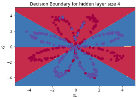
11.完事!开始跑模型,把结果得到的决策边界画出来
parameters = nn_model(X, Y, n_h = 4, num_iterations = 10000, print_cost=True)

# Plot the decision boundary
plot_decision_boundary(lambda x: predict(parameters, x.T), X, Y[0, :])
plt.title("Decision Boundary for hidden layer size " + str(4))
结束了得到下面这个图,和准确率90% ,雀食蟀,我只能说是雀食蟀
12.一个更进一步的对不同深度的网络的对比
plt.figure(figsize=(16, 32))
hidden_layer_sizes = [1, 2, 3, 4, 5, 10, 20]
for i, n_h in enumerate(hidden_layer_sizes):
    plt.subplot(5, 2, i+1)
    plt.title('Hidden Layer of size %d' % n_h)
    parameters = nn_model(X, Y, n_h, num_iterations = 5000)
    plot_decision_boundary(lambda x: predict(parameters, x.T), X, Y[0, :])
    predictions = predict(parameters, X)
    accuracy = float((np.dot(Y,predictions.T) + np.dot(1-Y,1-predictions.T))/float(Y.size)*100)
    print ("Accuracy for {} hidden units: {} %".format(n_h, accuracy))
分别用的1层、2层到20层来展示跑出来的结果,得到的准确率分别为
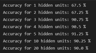
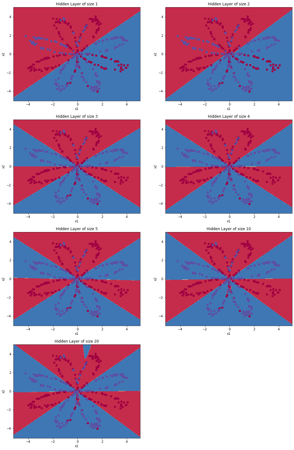
可以看出来:1.良好的分类结果并不是由线性模型简单增加层数就可以得到的;
2.较大的模型(具有更多隐藏单元)能够更好地拟合训练集;
3.最佳隐藏层大小似乎在n_h=5左右。事实上,这个值似乎与数据吻合得很好,也不会引起明显的过度拟合。
4.更深层的神经网络不一定能有更好的结果,因为有可能会带来过拟合的问题,所以后面我们需要加入正则化来避免这个问题,但正则化也会带来精度下降(方差减小而误差增大)的问题。
完结撒花~
