利用scikit-learn库中的数据集学习数据分类

　　工欲善其事，必先利其器。

1、安装环境：

pip install numpy scipy matplotlib scikit-learn -i https://pypi.tuna.tsinghua.edu.cn/simple

2、常规导库操作：

import  pandas as pd #倒库操作
import numpy as np

import sklearn
from sklearn import datasets #导入数据集合

3、应用数据集获取载入鸢尾花数据：

#读取分类的数据
iris = datasets.load_iris()

4、查看类型：

type(iris)
结果：
sklearn.utils._bunch.Bunch

5、查看数据：

iris
结果：
{'data': array([[5.1, 3.5, 1.4, 0.2],
        [4.9, 3. , 1.4, 0.2],
        [4.7, 3.2, 1.3, 0.2],
        [4.6, 3.1, 1.5, 0.2],
        [5. , 3.6, 1.4, 0.2],
        [5.4, 3.9, 1.7, 0.4],
        [4.6, 3.4, 1.4, 0.3],
        [5. , 3.4, 1.5, 0.2],
        [4.4, 2.9, 1.4, 0.2],
        [4.9, 3.1, 1.5, 0.1],
        [5.4, 3.7, 1.5, 0.2],
        [4.8, 3.4, 1.6, 0.2],
        [4.8, 3. , 1.4, 0.1],
        [4.3, 3. , 1.1, 0.1],
        [5.8, 4. , 1.2, 0.2],
        [5.7, 4.4, 1.5, 0.4],
        [5.4, 3.9, 1.3, 0.4],
        [5.1, 3.5, 1.4, 0.3],
        [5.7, 3.8, 1.7, 0.3],
        [5.1, 3.8, 1.5, 0.3],
        [5.4, 3.4, 1.7, 0.2],
        [5.1, 3.7, 1.5, 0.4],
        [4.6, 3.6, 1. , 0.2],
        [5.1, 3.3, 1.7, 0.5],
        [4.8, 3.4, 1.9, 0.2],
        [5. , 3. , 1.6, 0.2],
        [5. , 3.4, 1.6, 0.4],
        [5.2, 3.5, 1.5, 0.2],
        [5.2, 3.4, 1.4, 0.2],
        [4.7, 3.2, 1.6, 0.2],
        [4.8, 3.1, 1.6, 0.2],
        [5.4, 3.4, 1.5, 0.4],
        [5.2, 4.1, 1.5, 0.1],
        [5.5, 4.2, 1.4, 0.2],
        [4.9, 3.1, 1.5, 0.2],
        [5. , 3.2, 1.2, 0.2],
        [5.5, 3.5, 1.3, 0.2],
        [4.9, 3.6, 1.4, 0.1],
        [4.4, 3. , 1.3, 0.2],
        [5.1, 3.4, 1.5, 0.2],
        [5. , 3.5, 1.3, 0.3],
        [4.5, 2.3, 1.3, 0.3],
        [4.4, 3.2, 1.3, 0.2],
        [5. , 3.5, 1.6, 0.6],
        [5.1, 3.8, 1.9, 0.4],
        [4.8, 3. , 1.4, 0.3],
        [5.1, 3.8, 1.6, 0.2],
        [4.6, 3.2, 1.4, 0.2],
        [5.3, 3.7, 1.5, 0.2],
        [5. , 3.3, 1.4, 0.2],
        [7. , 3.2, 4.7, 1.4],
        [6.4, 3.2, 4.5, 1.5],
        [6.9, 3.1, 4.9, 1.5],
        [5.5, 2.3, 4. , 1.3],
        [6.5, 2.8, 4.6, 1.5],
        [5.7, 2.8, 4.5, 1.3],
        [6.3, 3.3, 4.7, 1.6],
        [4.9, 2.4, 3.3, 1. ],
        [6.6, 2.9, 4.6, 1.3],
        [5.2, 2.7, 3.9, 1.4],
        [5. , 2. , 3.5, 1. ],
        [5.9, 3. , 4.2, 1.5],
        [6. , 2.2, 4. , 1. ],
        [6.1, 2.9, 4.7, 1.4],
        [5.6, 2.9, 3.6, 1.3],
        [6.7, 3.1, 4.4, 1.4],
        [5.6, 3. , 4.5, 1.5],
        [5.8, 2.7, 4.1, 1. ],
        [6.2, 2.2, 4.5, 1.5],
        [5.6, 2.5, 3.9, 1.1],
        [5.9, 3.2, 4.8, 1.8],
        [6.1, 2.8, 4. , 1.3],
        [6.3, 2.5, 4.9, 1.5],
        [6.1, 2.8, 4.7, 1.2],
        [6.4, 2.9, 4.3, 1.3],
        [6.6, 3. , 4.4, 1.4],
        [6.8, 2.8, 4.8, 1.4],
        [6.7, 3. , 5. , 1.7],
        [6. , 2.9, 4.5, 1.5],
        [5.7, 2.6, 3.5, 1. ],
        [5.5, 2.4, 3.8, 1.1],
        [5.5, 2.4, 3.7, 1. ],
        [5.8, 2.7, 3.9, 1.2],
        [6. , 2.7, 5.1, 1.6],
        [5.4, 3. , 4.5, 1.5],
        [6. , 3.4, 4.5, 1.6],
        [6.7, 3.1, 4.7, 1.5],
        [6.3, 2.3, 4.4, 1.3],
        [5.6, 3. , 4.1, 1.3],
        [5.5, 2.5, 4. , 1.3],
        [5.5, 2.6, 4.4, 1.2],
        [6.1, 3. , 4.6, 1.4],
        [5.8, 2.6, 4. , 1.2],
        [5. , 2.3, 3.3, 1. ],
        [5.6, 2.7, 4.2, 1.3],
        [5.7, 3. , 4.2, 1.2],
        [5.7, 2.9, 4.2, 1.3],
        [6.2, 2.9, 4.3, 1.3],
        [5.1, 2.5, 3. , 1.1],
        [5.7, 2.8, 4.1, 1.3],
        [6.3, 3.3, 6. , 2.5],
        [5.8, 2.7, 5.1, 1.9],
        [7.1, 3. , 5.9, 2.1],
        [6.3, 2.9, 5.6, 1.8],
        [6.5, 3. , 5.8, 2.2],
        [7.6, 3. , 6.6, 2.1],
        [4.9, 2.5, 4.5, 1.7],
        [7.3, 2.9, 6.3, 1.8],
        [6.7, 2.5, 5.8, 1.8],
        [7.2, 3.6, 6.1, 2.5],
        [6.5, 3.2, 5.1, 2. ],
        [6.4, 2.7, 5.3, 1.9],
        [6.8, 3. , 5.5, 2.1],
        [5.7, 2.5, 5. , 2. ],
        [5.8, 2.8, 5.1, 2.4],
        [6.4, 3.2, 5.3, 2.3],
        [6.5, 3. , 5.5, 1.8],
        [7.7, 3.8, 6.7, 2.2],
        [7.7, 2.6, 6.9, 2.3],
        [6. , 2.2, 5. , 1.5],
        [6.9, 3.2, 5.7, 2.3],
        [5.6, 2.8, 4.9, 2. ],
        [7.7, 2.8, 6.7, 2. ],
        [6.3, 2.7, 4.9, 1.8],
        [6.7, 3.3, 5.7, 2.1],
        [7.2, 3.2, 6. , 1.8],
        [6.2, 2.8, 4.8, 1.8],
        [6.1, 3. , 4.9, 1.8],
        [6.4, 2.8, 5.6, 2.1],
        [7.2, 3. , 5.8, 1.6],
        [7.4, 2.8, 6.1, 1.9],
        [7.9, 3.8, 6.4, 2. ],
        [6.4, 2.8, 5.6, 2.2],
        [6.3, 2.8, 5.1, 1.5],
        [6.1, 2.6, 5.6, 1.4],
        [7.7, 3. , 6.1, 2.3],
        [6.3, 3.4, 5.6, 2.4],
        [6.4, 3.1, 5.5, 1.8],
        [6. , 3. , 4.8, 1.8],
        [6.9, 3.1, 5.4, 2.1],
        [6.7, 3.1, 5.6, 2.4],
        [6.9, 3.1, 5.1, 2.3],
        [5.8, 2.7, 5.1, 1.9],
        [6.8, 3.2, 5.9, 2.3],
        [6.7, 3.3, 5.7, 2.5],
        [6.7, 3. , 5.2, 2.3],
        [6.3, 2.5, 5. , 1.9],
        [6.5, 3. , 5.2, 2. ],
        [6.2, 3.4, 5.4, 2.3],
        [5.9, 3. , 5.1, 1.8]]),
 'target': array([0, 0, 0, 0, 0, 0, 0, 0, 0, 0, 0, 0, 0, 0, 0, 0, 0, 0, 0, 0, 0, 0,
        0, 0, 0, 0, 0, 0, 0, 0, 0, 0, 0, 0, 0, 0, 0, 0, 0, 0, 0, 0, 0, 0,
        0, 0, 0, 0, 0, 0, 1, 1, 1, 1, 1, 1, 1, 1, 1, 1, 1, 1, 1, 1, 1, 1,
        1, 1, 1, 1, 1, 1, 1, 1, 1, 1, 1, 1, 1, 1, 1, 1, 1, 1, 1, 1, 1, 1,
        1, 1, 1, 1, 1, 1, 1, 1, 1, 1, 1, 1, 2, 2, 2, 2, 2, 2, 2, 2, 2, 2,
        2, 2, 2, 2, 2, 2, 2, 2, 2, 2, 2, 2, 2, 2, 2, 2, 2, 2, 2, 2, 2, 2,
        2, 2, 2, 2, 2, 2, 2, 2, 2, 2, 2, 2, 2, 2, 2, 2, 2, 2]),
 'frame': None,
 'target_names': array(['setosa', 'versicolor', 'virginica'], dtype='<U10'),
 'DESCR': '.. _iris_dataset:\n\nIris plants dataset\n--------------------\n\n**Data Set Characteristics:**\n\n    :Number of Instances: 150 (50 in each of three classes)\n    :Number of Attributes: 4 numeric, predictive attributes and the class\n    :Attribute Information:\n        - sepal length in cm\n        - sepal width in cm\n        - petal length in cm\n        - petal width in cm\n        - class:\n                - Iris-Setosa\n                - Iris-Versicolour\n                - Iris-Virginica\n                \n    :Summary Statistics:\n\n    ============== ==== ==== ======= ===== ====================\n                    Min  Max   Mean    SD   Class Correlation\n    ============== ==== ==== ======= ===== ====================\n    sepal length:   4.3  7.9   5.84   0.83    0.7826\n    sepal width:    2.0  4.4   3.05   0.43   -0.4194\n    petal length:   1.0  6.9   3.76   1.76    0.9490  (high!)\n    petal width:    0.1  2.5   1.20   0.76    0.9565  (high!)\n    ============== ==== ==== ======= ===== ====================\n\n    :Missing Attribute Values: None\n    :Class Distribution: 33.3% for each of 3 classes.\n    :Creator: R.A. Fisher\n    :Donor: Michael Marshall (MARSHALL%PLU@io.arc.nasa.gov)\n    :Date: July, 1988\n\nThe famous Iris database, first used by Sir R.A. Fisher. The dataset is taken\nfrom Fisher\'s paper. Note that it\'s the same as in R, but not as in the UCI\nMachine Learning Repository, which has two wrong data points.\n\nThis is perhaps the best known database to be found in the\npattern recognition literature.  Fisher\'s paper is a classic in the field and\nis referenced frequently to this day.  (See Duda & Hart, for example.)  The\ndata set contains 3 classes of 50 instances each, where each class refers to a\ntype of iris plant.  One class is linearly separable from the other 2; the\nlatter are NOT linearly separable from each other.\n\n.. topic:: References\n\n   - Fisher, R.A. "The use of multiple measurements in taxonomic problems"\n     Annual Eugenics, 7, Part II, 179-188 (1936); also in "Contributions to\n     Mathematical Statistics" (John Wiley, NY, 1950).\n   - Duda, R.O., & Hart, P.E. (1973) Pattern Classification and Scene Analysis.\n     (Q327.D83) John Wiley & Sons.  ISBN 0-471-22361-1.  See page 218.\n   - Dasarathy, B.V. (1980) "Nosing Around the Neighborhood: A New System\n     Structure and Classification Rule for Recognition in Partially Exposed\n     Environments".  IEEE Transactions on Pattern Analysis and Machine\n     Intelligence, Vol. PAMI-2, No. 1, 67-71.\n   - Gates, G.W. (1972) "The Reduced Nearest Neighbor Rule".  IEEE Transactions\n     on Information Theory, May 1972, 431-433.\n   - See also: 1988 MLC Proceedings, 54-64.  Cheeseman et al"s AUTOCLASS II\n     conceptual clustering system finds 3 classes in the data.\n   - Many, many more ...',
 'feature_names': ['sepal length (cm)',
  'sepal width (cm)',
  'petal length (cm)',
  'petal width (cm)'],
 'filename': 'iris.csv',
 'data_module': 'sklearn.datasets.data'}

　　后面是数据的特征：主要包括data, target, frame, target_names, feature_names, filename等。

6、查看data类型：

type(iris.data)
结果：
numpy.ndarray

7、查看target数据

iris.target
结果：
array([0, 0, 0, 0, 0, 0, 0, 0, 0, 0, 0, 0, 0, 0, 0, 0, 0, 0, 0, 0, 0, 0,
       0, 0, 0, 0, 0, 0, 0, 0, 0, 0, 0, 0, 0, 0, 0, 0, 0, 0, 0, 0, 0, 0,
       0, 0, 0, 0, 0, 0, 1, 1, 1, 1, 1, 1, 1, 1, 1, 1, 1, 1, 1, 1, 1, 1,
       1, 1, 1, 1, 1, 1, 1, 1, 1, 1, 1, 1, 1, 1, 1, 1, 1, 1, 1, 1, 1, 1,
       1, 1, 1, 1, 1, 1, 1, 1, 1, 1, 1, 1, 2, 2, 2, 2, 2, 2, 2, 2, 2, 2,
       2, 2, 2, 2, 2, 2, 2, 2, 2, 2, 2, 2, 2, 2, 2, 2, 2, 2, 2, 2, 2, 2,
       2, 2, 2, 2, 2, 2, 2, 2, 2, 2, 2, 2, 2, 2, 2, 2, 2, 2])

8、查看target类型

type(iris.target)
结果：
numpy.ndarray

9、查看target的属性，也就是表的表头

iris.target_names
结果：
array(['setosa', 'versicolor', 'virginica'], dtype='<U10')

10、查看feature_names

iris.feature_names
结果：
['sepal length (cm)',
 'sepal width (cm)',
 'petal length (cm)',
 'petal width (cm)']

11、获取鸢尾花数据，并查看

df_iris = pd.DataFrame(iris.data, columns = iris.feature_names)
df_iris

　　对鸢尾花数据也可以直接获取到dataframe数据

#可以直接返回特征和目标变量
x,y = load_iris(return_X_y=True)
#可以直接返回pandas的DataFrame
x,y = load_iris(return_X_y=True , as_frame=True)
x.head()
y.head()

　　别看了，我错误的认为load_boston()方法中也有as_frame参数，然而并没有，CTMD，这也太不严谨了，都免费给你用，还想咋的，还不错。需要多看文档啊。

结果：

    sepal length (cm)    sepal width (cm)    petal length (cm)    petal width (cm)
0    5.1    3.5    1.4    0.2
1    4.9    3.0    1.4    0.2
2    4.7    3.2    1.3    0.2
3    4.6    3.1    1.5    0.2
4    5.0    3.6    1.4    0.2
...    ...    ...    ...    ...
145    6.7    3.0    5.2    2.3
146    6.3    2.5    5.0    1.9
147    6.5    3.0    5.2    2.0
148    6.2    3.4    5.4    2.3
149    5.9    3.0    5.1    1.8
150 rows × 4 columns

注意：此处的数据有省略，150条数据，只是显示了10条，省略了140条

12、操作数据，添加target列数据，并查看

df_iris["target"] = iris.target
df_iris

结果：

sepal length (cm)    sepal width (cm)    petal length (cm)    petal width (cm)    target
0    5.1    3.5    1.4    0.2    0
1    4.9    3.0    1.4    0.2    0
2    4.7    3.2    1.3    0.2    0
3    4.6    3.1    1.5    0.2    0
4    5.0    3.6    1.4    0.2    0
...    ...    ...    ...    ...    ...
145    6.7    3.0    5.2    2.3    2
146    6.3    2.5    5.0    1.9    2
147    6.5    3.0    5.2    2.0    2
148    6.2    3.4    5.4    2.3    2
149    5.9    3.0    5.1    1.8    2
150 rows × 5 columns

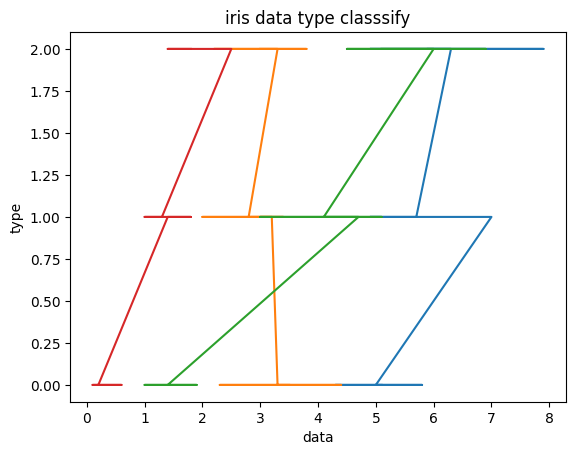
13、绘图

#导入数据和标签
data_x = data.data
data_y = data.target

from matplotlib import pyplot as plt
%matplotlib inline

plt.plot(data_x, data_y)
plt.title("iris data type classify")
plt.xlabel('data')
plt.ylabel('type')

结果：

你学废了吗