How a Kalman filter works, in pictures中英文
How a Kalman filter works, in pictures | Bzarg
How a Kalman filter works, in pictures
I have to tell you about the Kalman filter, because what it does is pretty damn amazing.
Surprisingly few software engineers and scientists seem to know about it, and that makes me sad because it is such a general and powerful tool for combining information in the presence of uncertainty. At times its ability to extract accurate information seems almost magical— and if it sounds like I’m talking this up too much, then take a look at this previously posted video where I demonstrate a Kalman filter figuring out the orientation of a free-floating body by looking at its velocity. Totally neat!
What is it?
You can use a Kalman filter in any place where you have uncertain information about some dynamic system, and you can make an educated guess about what the system is going to do next. Even if messy reality comes along and interferes with the clean motion you guessed about, the Kalman filter will often do a very good job of figuring out what actually happened. And it can take advantage of correlations between crazy phenomena that you maybe wouldn’t have thought to exploit!
Kalman filters are ideal for systems which are continuously changing. They have the advantage that they are light on memory (they don’t need to keep any history other than the previous state), and they are very fast, making them well suited for real time problems and embedded systems.
The math for implementing the Kalman filter appears pretty scary and opaque in most places you find on Google. That’s a bad state of affairs, because the Kalman filter is actually super simple and easy to understand if you look at it in the right way. Thus it makes a great article topic, and I will attempt to illuminate it with lots of clear, pretty pictures and colors. The prerequisites are simple; all you need is a basic understanding of probability and matrices.
I’ll start with a loose example of the kind of thing a Kalman filter can solve, but if you want to get right to the shiny pictures and math, feel free to jump ahead.
What can we do with a Kalman filter?
Let’s make a toy example: You’ve built a little robot that can wander around in the woods, and the robot needs to know exactly where it is so that it can navigate.

We’ll say our robot has a state , which is just a position and a velocity:
Note that the state is just a list of numbers about the underlying configuration of your system; it could be anything. In our example it’s position and velocity, but it could be data about the amount of fluid in a tank, the temperature of a car engine, the position of a user’s finger on a touchpad, or any number of things you need to keep track of.
Our robot also has a GPS sensor, which is accurate to about 10 meters, which is good, but it needs to know its location more precisely than 10 meters. There are lots of gullies and cliffs in these woods, and if the robot is wrong by more than a few feet, it could fall off a cliff. So GPS by itself is not good enough.
We might also know something about how the robot moves: It knows the commands sent to the wheel motors, and its knows that if it’s headed in one direction and nothing interferes, at the next instant it will likely be further along that same direction. But of course it doesn’t know everything about its motion: It might be buffeted by the wind, the wheels might slip a little bit, or roll over bumpy terrain; so the amount the wheels have turned might not exactly represent how far the robot has actually traveled, and the prediction won’t be perfect.
The GPS sensor tells us something about the state, but only indirectly, and with some uncertainty or inaccuracy. Our prediction tells us something about how the robot is moving, but only indirectly, and with some uncertainty or inaccuracy.
But if we use all the information available to us, can we get a better answer than either estimate would give us by itself? Of course the answer is yes, and that’s what a Kalman filter is for.
How a Kalman filter sees your problem
Let’s look at the landscape we’re trying to interpret. We’ll continue with a simple state having only position and velocity.
We don’t know what the actual position and velocity are; there are a whole range of possible combinations of position and velocity that might be true, but some of them are more likely than others:
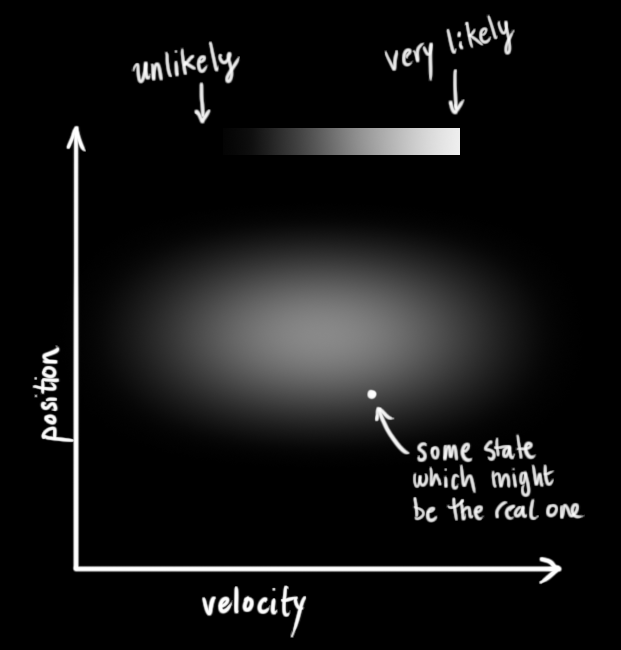
The Kalman filter assumes that both variables (postion and velocity, in our case) are random and Gaussian distributed. Each variable has a mean value , which is the center of the random distribution (and its most likely state), and a variance , which is the uncertainty:
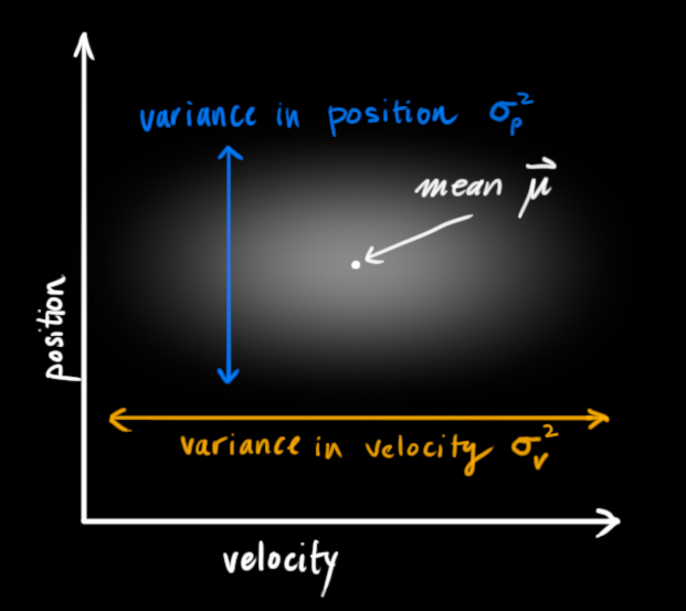
In the above picture, position and velocity are uncorrelated, which means that the state of one variable tells you nothing about what the other might be.
The example below shows something more interesting: Position and velocity are correlated. The likelihood of observing a particular position depends on what velocity you have:
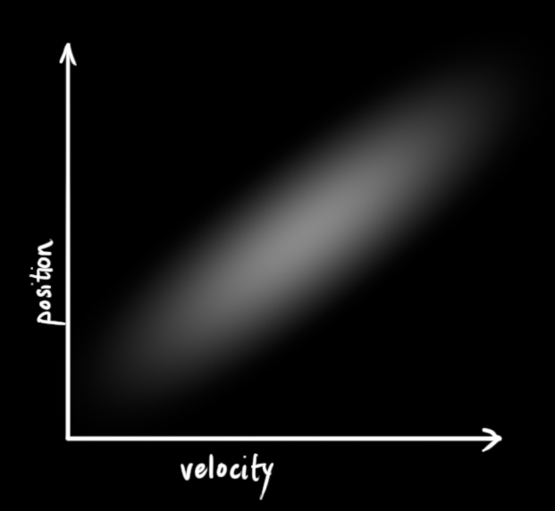 This kind of situation might arise if, for example, we are estimating a new position based on an old one. If our velocity was high, we probably moved farther, so our position will be more distant. If we’re moving slowly, we didn’t get as far.
This kind of relationship is really important to keep track of, because it gives us more information: One measurement tells us something about what the others could be. And that’s the goal of the Kalman filter, we want to squeeze as much information from our uncertain measurements as we possibly can!
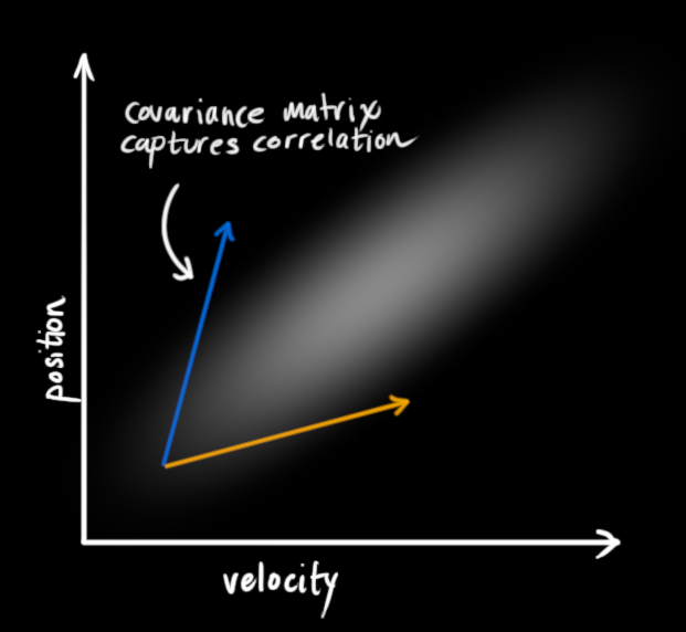
This correlation is captured by something called a covariance matrix. In short, each element of the matrix is the degree of correlation between the ith state variable and the jth state variable. (You might be able to guess that the covariance matrix is symmetric, which means that it doesn’t matter if you swap i and j). Covariance matrices are often labelled “”, so we call their elements “”.
Describing the problem with matrices
We’re modeling our knowledge about the state as a Gaussian blob, so we need two pieces of information at time : We’ll call our best estimate (the mean, elsewhere named ), and its covariance matrix .
(Of course we are using only position and velocity here, but it’s useful to remember that the state can contain any number of variables, and represent anything you want).
Next, we need some way to look at the current state (at time k-1) and predict the next state at time k. Remember, we don’t know which state is the “real” one, but our prediction function doesn’t care. It just works on all of them, and gives us a new distribution:
 We can represent this prediction step with a matrix, :
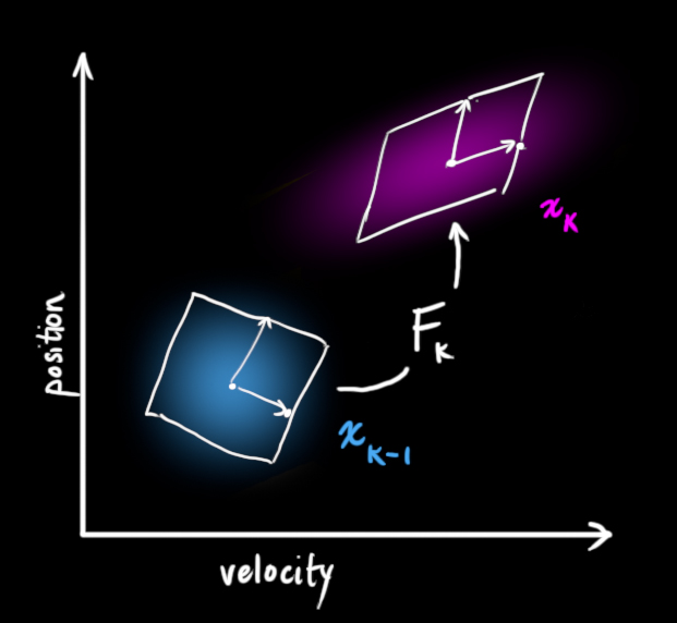 It takes every point in our original estimate and moves it to a new predicted location, which is where the system would move if that original estimate was the right one.
Let’s apply this. How would we use a matrix to predict the position and velocity at the next moment in the future? We’ll use a really basic kinematic formula: In other words:
We now have a prediction matrix which gives us our next state, but we still don’t know how to update the covariance matrix.
This is where we need another formula. If we multiply every point in a distribution by a matrix , then what happens to its covariance matrix ?
Well, it’s easy. I’ll just give you the identity:
So combining with equation :
External influence
We haven’t captured everything, though. There might be some changes that aren’t related to the state itself— the outside world could be affecting the system.
For example, if the state models the motion of a train, the train operator might push on the throttle, causing the train to accelerate. Similarly, in our robot example, the navigation software might issue a command to turn the wheels or stop. If we know this additional information about what’s going on in the world, we could stuff it into a vector called , do something with it, and add it to our prediction as a correction.
Let’s say we know the expected acceleration due to the throttle setting or control commands. From basic kinematics we get: In matrix form:
is called the control matrix and the control vector. (For very simple systems with no external influence, you could omit these).
Let’s add one more detail. What happens if our prediction is not a 100% accurate model of what’s actually going on?
External uncertainty
Everything is fine if the state evolves based on its own properties. Everything is still fine if the state evolves based on external forces, so long as we know what those external forces are.
But what about forces that we don’t know about? If we’re tracking a quadcopter, for example, it could be buffeted around by wind. If we’re tracking a wheeled robot, the wheels could slip, or bumps on the ground could slow it down. We can’t keep track of these things, and if any of this happens, our prediction could be off because we didn’t account for those extra forces.
We can model the uncertainty associated with the “world” (i.e. things we aren’t keeping track of) by adding some new uncertainty after every prediction step:
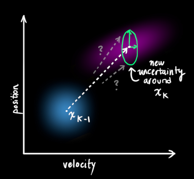
Every state in our original estimate could have moved to a range of states. Because we like Gaussian blobs so much, we’ll say that each point in is moved to somewhere inside a Gaussian blob with covariance . Another way to say this is that we are treating the untracked influences as noise with covariance .
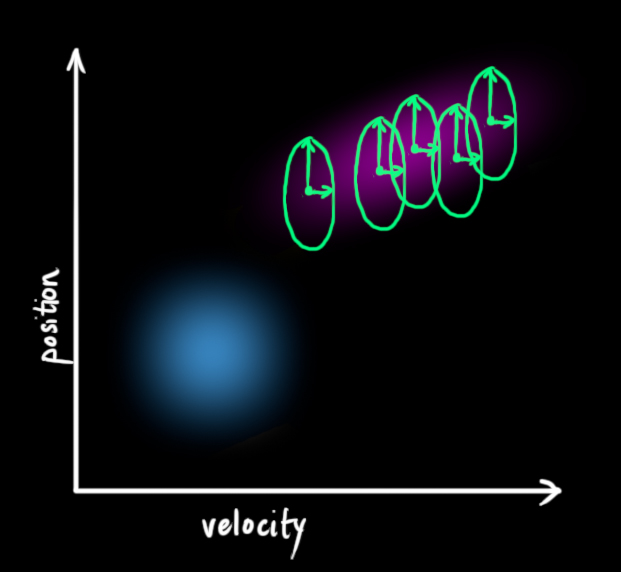 This produces a new Gaussian blob, with a different covariance (but the same mean):
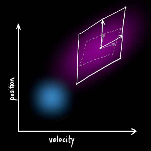
We get the expanded covariance by simply adding , giving our complete expression for the prediction step:
In other words, the new best estimate is a prediction made from previous best estimate, plus a correction for known external influences.
And the new uncertainty is predicted from the old uncertainty, with some additional uncertainty from the environment.
All right, so that’s easy enough. We have a fuzzy estimate of where our system might be, given by and . What happens when we get some data from our sensors?
Refining the estimate with measurements
We might have several sensors which give us information about the state of our system. For the time being it doesn’t matter what they measure; perhaps one reads position and the other reads velocity. Each sensor tells us something indirect about the state— in other words, the sensors operate on a state and produce a set of readings.
 Notice that the units and scale of the reading might not be the same as the units and scale of the state we’re keeping track of. You might be able to guess where this is going: We’ll model the sensors with a matrix, .
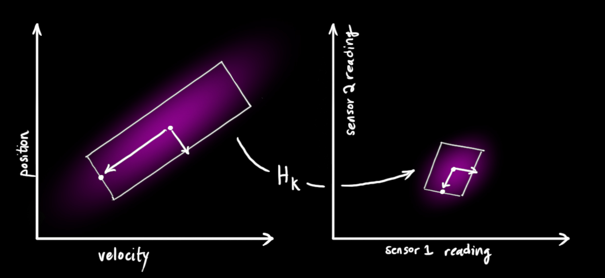
We can figure out the distribution of sensor readings we’d expect to see in the usual way:
One thing that Kalman filters are great for is dealing with sensor noise. In other words, our sensors are at least somewhat unreliable, and every state in our original estimate might result in a range of sensor readings.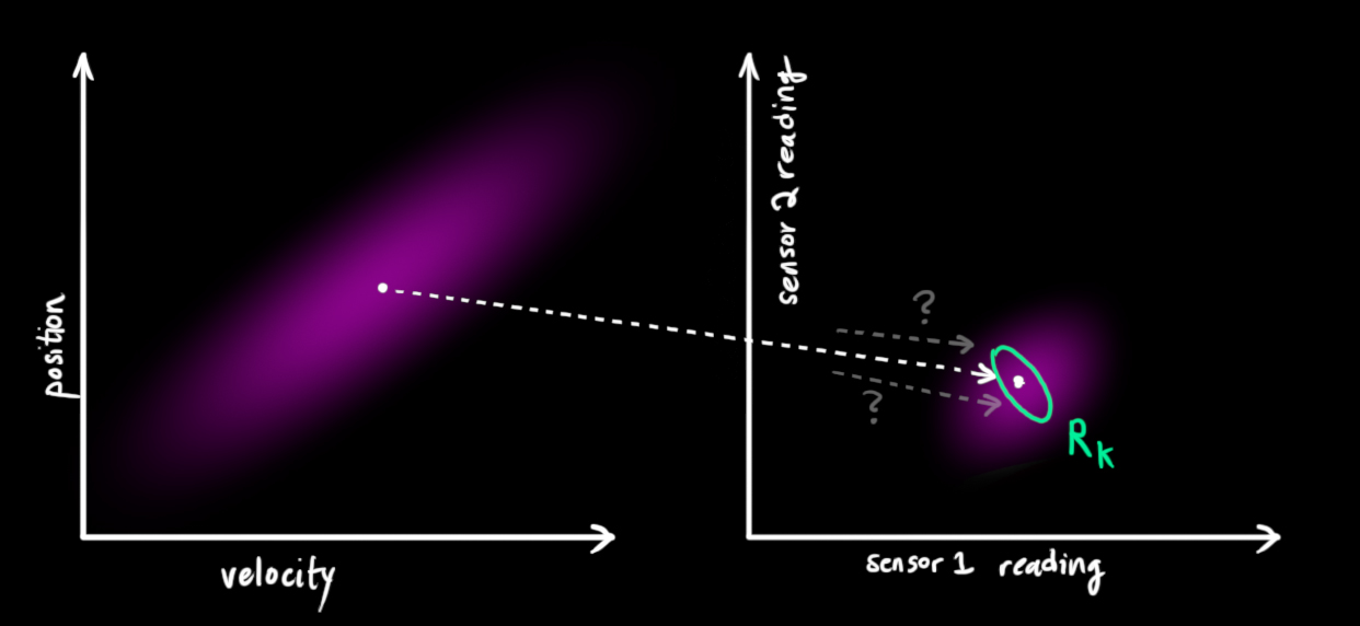
From each reading we observe, we might guess that our system was in a particular state. But because there is uncertainty, some states are more likely than others to have have produced the reading we saw: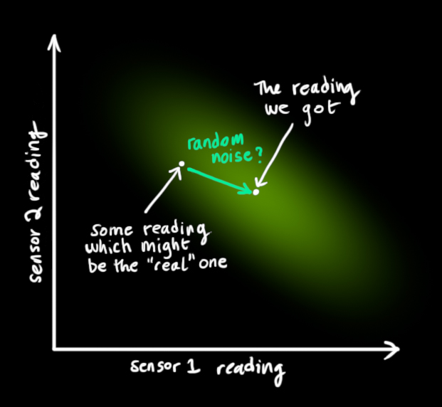
We’ll call the covariance of this uncertainty (i.e. of the sensor noise) . The distribution has a mean equal to the reading we observed, which we’ll call .
So now we have two Gaussian blobs: One surrounding the mean of our transformed prediction, and one surrounding the actual sensor reading we got.
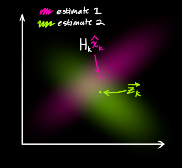
We must try to reconcile our guess about the readings we’d see based on the predicted state (pink) with a different guess based on our sensor readings (green) that we actually observed.
So what’s our new most likely state? For any possible reading , we have two associated probabilities: (1) The probability that our sensor reading is a (mis-)measurement of , and (2) the probability that our previous estimate thinks is the reading we should see.
If we have two probabilities and we want to know the chance that both are true, we just multiply them together. So, we take the two Gaussian blobs and multiply them:
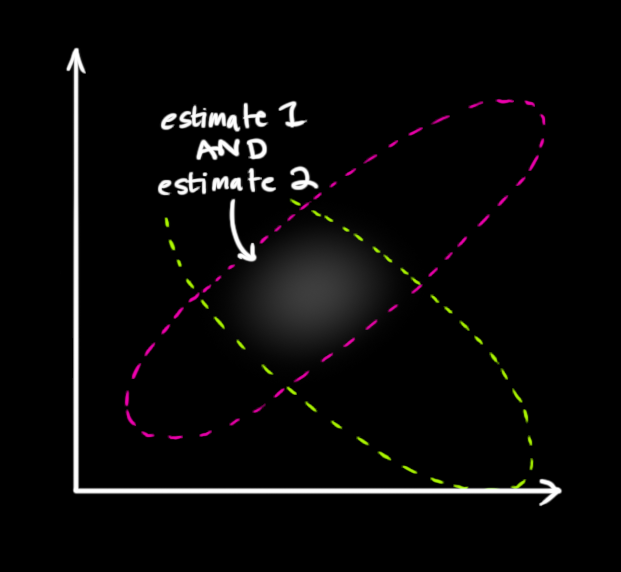
What we’re left with is the overlap, the region where both blobs are bright/likely. And it’s a lot more precise than either of our previous estimates. The mean of this distribution is the configuration for which both estimates are most likely, and is therefore the best guess of the true configuration given all the information we have.
Hmm. This looks like another Gaussian blob.
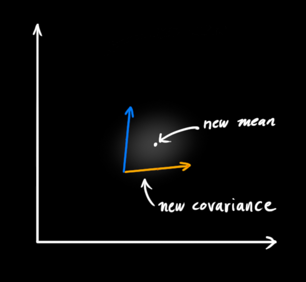
As it turns out, when you multiply two Gaussian blobs with separate means and covariance matrices, you get a new Gaussian blob with its own mean and covariance matrix! Maybe you can see where this is going: There’s got to be a formula to get those new parameters from the old ones!
Combining Gaussians
Let’s find that formula. It’s easiest to look at this first in one dimension. A 1D Gaussian bell curve with variance and mean is defined as:
We want to know what happens when you multiply two Gaussian curves together. The blue curve below represents the (unnormalized) intersection of the two Gaussian populations:
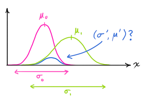
You can substitute equation into equation and do some algebra (being careful to renormalize, so that the total probability is 1) to obtain:
We can simplify by factoring out a little piece and calling it :
Take note of how you can take your previous estimate and add something to make a new estimate. And look at how simple that formula is!
But what about a matrix version? Well, let’s just re-write equations and in matrix form. If is the covariance matrix of a Gaussian blob, and its mean along each axis, then:
is a matrix called the Kalman gain, and we’ll use it in just a moment.
Easy! We’re almost finished!
Putting it all together
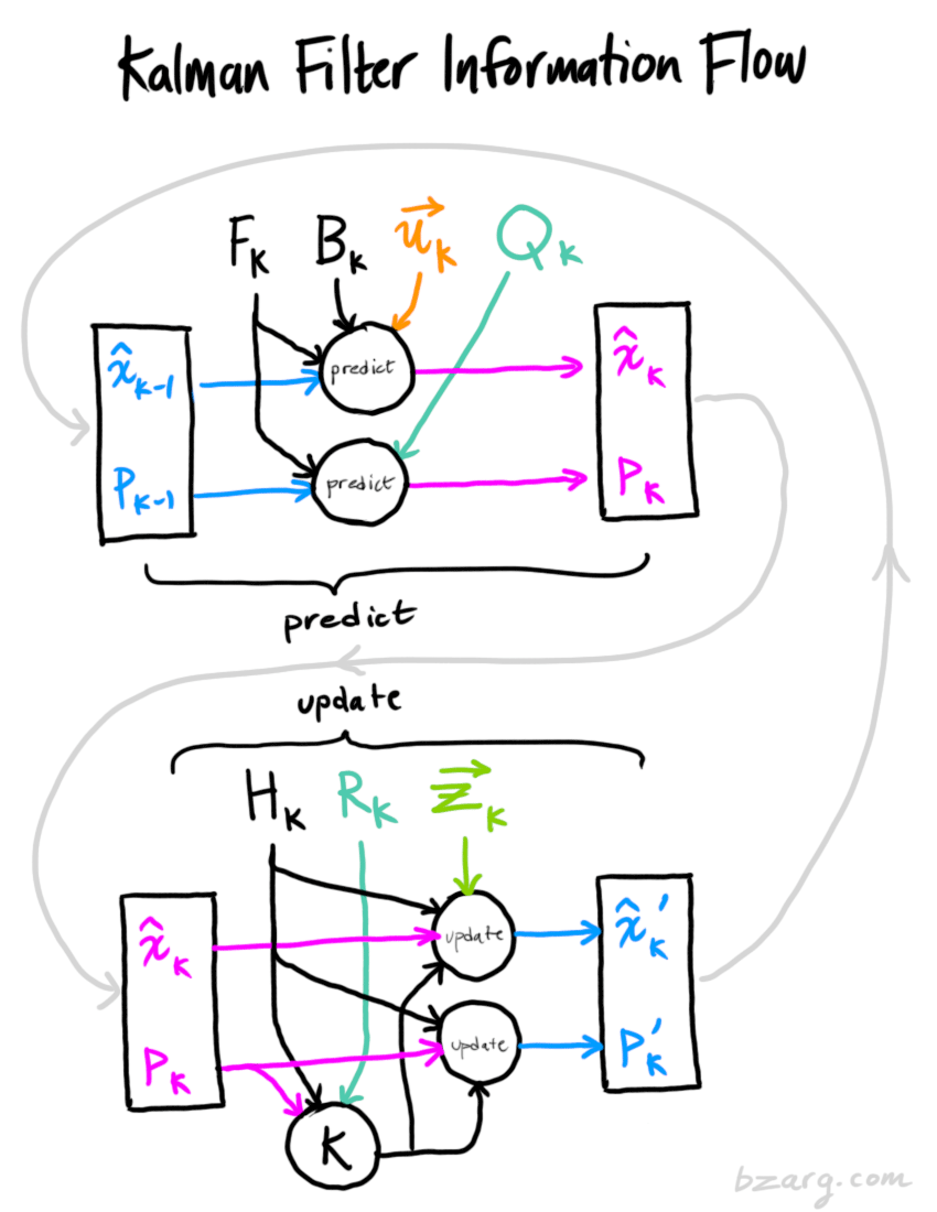
We have two distributions: The predicted measurement with , and the observed measurement with . We can just plug these into equation to find their overlap: And from , the Kalman gain is: We can knock an off the front of every term in and (note that one is hiding inside ), and an off the end of all terms in the equation for . …giving us the complete equations for the update step.
And that’s it! is our new best estimate, and we can go on and feed it (along with ) back into another round of predict or update as many times as we like.
Wrapping up
Of all the math above, all you need to implement are equations , and . (Or if you forget those, you could re-derive everything from equations and .)
This will allow you to model any linear system accurately. For nonlinear systems, we use the extended Kalman filter, which works by simply linearizing the predictions and measurements about their mean. (I may do a second write-up on the EKF in the future).
If I’ve done my job well, hopefully someone else out there will realize how cool these things are and come up with an unexpected new place to put them into action.
Some credit and referral should be given to this fine document, which uses a similar approach involving overlapping Gaussians. More in-depth derivations can be found there, for the curious.
详解卡尔曼滤波原理_清风莞尔的博客-CSDN博客_卡尔曼滤波原理
在网上看了不少与卡尔曼滤波相关的博客、论文,要么是只谈理论、缺乏感性,或者有感性认识,缺乏理论推导。能兼顾二者的少之又少,直到我看到了国外的一篇博文,真的惊艳到我了,不得不佩服作者这种细致入微的精神,翻译过来跟大家分享一下,原文链接:http://www.bzarg.com/p/how-a-kalman-filter-works-in-pictures/
我不得不说说卡尔曼滤波,因为它能做到的事情简直让人惊叹!意外的是很少有软件工程师和科学家对对它有所了解,这让我感到沮丧,因为卡尔曼滤波是一个如此强大的工具,能够在不确定性中融合信息,与此同时,它提取精确信息的能力看起来不可思议。
什么是卡尔曼滤波?
你可以在任何含有不确定信息的动态系统中使用卡尔曼滤波,对系统下一步的走向做出有根据的预测,即使伴随着各种干扰,卡尔曼滤波总是能指出真实发生的情况。
在连续变化的系统中使用卡尔曼滤波是非常理想的,它具有占用内存小的优点(除了前一个状态量外,不需要保留其它历史数据),并且速度很快,很适合应用于实时问题和嵌入式系统。
在Google上找到的大多数关于实现卡尔曼滤波的数学公式看起来有点晦涩难懂,这个状况有点糟糕。实际上,如果以正确的方式看待它,卡尔曼滤波是非常简单和容易理解的,下面我将用漂亮的图片和色彩清晰的阐述它,你只需要懂一些基本的概率和矩阵的知识就可以了。
我们能用卡尔曼滤波做什么?
用玩具举例:你开发了一个可以在树林里到处跑的小机器人,这个机器人需要知道它所在的确切位置才能导航。

我们可以说机器人有一个状态 ,表示位置和速度:
注意这个状态只是关于这个系统基本属性的一堆数字,它可以是任何其它的东西。在这个例子中是位置和速度,它也可以是一个容器中液体的总量,汽车发动机的温度,用户手指在触摸板上的位置坐标,或者任何你需要跟踪的信号。
这个机器人带有GPS,精度大约为10米,还算不错,但是,它需要将自己的位置精确到10米以内。树林里有很多沟壑和悬崖,如果机器人走错了一步,就有可能掉下悬崖,所以只有GPS是不够的。

或许我们知道一些机器人如何运动的信息:例如,机器人知道发送给电机的指令,知道自己是否在朝一个方向移动并且没有人干预,在下一个状态,机器人很可能朝着相同的方向移动。当然,机器人对自己的运动是一无所知的:它可能受到风吹的影响,轮子方向偏了一点,或者遇到不平的地面而翻倒。所以,轮子转过的长度并不能精确表示机器人实际行走的距离,预测也不是很完美。
GPS 传感器告诉了我们一些状态信息,我们的预测告诉了我们机器人会怎样运动,但都只是间接的,并且伴随着一些不确定和不准确性。但是,如果使用所有对我们可用的信息,我们能得到一个比任何依据自身估计更好的结果吗?回答当然是YES,这就是卡尔曼滤波的用处。
卡尔曼滤波是如何看到你的问题的
下面我们继续以只有位置和速度这两个状态的简单例子做解释。
我们并不知道实际的位置和速度,它们之间有很多种可能正确的组合,但其中一些的可能性要大于其它部分:

卡尔曼滤波假设两个变量(位置和速度,在这个例子中)都是随机的,并且服从高斯分布。每个变量都有一个均值 μ,表示随机分布的中心(最可能的状态),以及方差 ,表示不确定性。

在上图中,位置和速度是不相关的,这意味着由其中一个变量的状态无法推测出另一个变量可能的值。下面的例子更有趣:位置和速度是相关的,观测特定位置的可能性取决于当前的速度:

这种情况是有可能发生的,例如,我们基于旧的位置来估计新位置。如果速度过高,我们可能已经移动很远了。如果缓慢移动,则距离不会很远。跟踪这种关系是非常重要的,因为它带给我们更多的信息:其中一个测量值告诉了我们其它变量可能的值,这就是卡尔曼滤波的目的,尽可能地在包含不确定性的测量数据中提取更多信息!
这种相关性用协方差矩阵来表示,简而言之,矩阵中的每个元素 表示第 i 个和第 j 个状态变量之间的相关度。(你可能已经猜到协方差矩阵是一个对称矩阵,这意味着可以任意交换 i 和 j)。协方差矩阵通常用“
”来表示,其中的元素则表示为“
”。

使用矩阵来描述问题
我们基于高斯分布来建立状态变量,所以在时刻 k 需要两个信息:最佳估计 (即均值,其它地方常用 μ 表示),以及协方差矩阵
。
(当然,在这里我们只用到了位置和速度,实际上这个状态可以包含多个变量,代表任何你想表示的信息)。接下来,我们需要根据当前状态(k-1 时刻)来预测下一状态(k 时刻)。记住,我们并不知道对下一状态的所有预测中哪个是“真实”的,但我们的预测函数并不在乎。它对所有的可能性进行预测,并给出新的高斯分布。

我们可以用矩阵 来表示这个预测过程:

它将我们原始估计中的每个点都移动到了一个新的预测位置,如果原始估计是正确的话,这个新的预测位置就是系统下一步会移动到的位置。那我们又如何用矩阵来预测下一个时刻的位置和速度呢?下面用一个基本的运动学公式来表示:

现在,我们有了一个预测矩阵来表示下一时刻的状态,但是,我们仍然不知道怎么更新协方差矩阵。此时,我们需要引入另一个公式,如果我们将分布中的每个点都乘以矩阵 A,那么它的协方差矩阵 会怎样变化呢?很简单,下面给出公式:

结合方程(4)和(3)得到:

外部控制量
我们并没有捕捉到一切信息,可能存在外部因素会对系统进行控制,带来一些与系统自身状态没有相关性的改变。
以火车的运动状态模型为例,火车司机可能会操纵油门,让火车加速。相同地,在我们机器人这个例子中,导航软件可能会发出一个指令让轮子转向或者停止。如果知道这些额外的信息,我们可以用一个向量
假设由于油门的设置或控制命令,我们知道了期望的加速度

以矩阵的形式表示就是:

称为控制矩阵,

外部干扰
如果这些状态量是基于系统自身的属性或者已知的外部控制作用来变化的,则不会出现什么问题。
但是,如果存在未知的干扰呢?例如,假设我们跟踪一个四旋翼飞行器,它可能会受到风的干扰,如果我们跟踪一个轮式机器人,轮子可能会打滑,或者路面上的小坡会让它减速。这样的话我们就不能继续对这些状态进行跟踪,如果没有把这些外部干扰考虑在内,我们的预测就会出现偏差。
在每次预测之后,我们可以添加一些新的不确定性来建立这种与“外界”(即我们没有跟踪的干扰)之间的不确定性模型:

原始估计中的每个状态变量更新到新的状态后,仍然服从高斯分布。我们可以说


这产生了具有不同协方差(但是具有相同的均值)的新的高斯分布。

我们通过简单地添加

由上式可知,新的最优估计是根据上一最优估计预测得到的,并加上已知外部控制量的修正。
而新的不确定性由上一不确定性预测得到,并加上外部环境的干扰。
好了,我们对系统可能的动向有了一个模糊的估计,用

用测量值来修正估计值
我们可能会有多个传感器来测量系统当前的状态,哪个传感器具体测量的是哪个状态变量并不重要,也许一个是测量位置,一个是测量速度,每个传感器间接地告诉了我们一些状态信息。
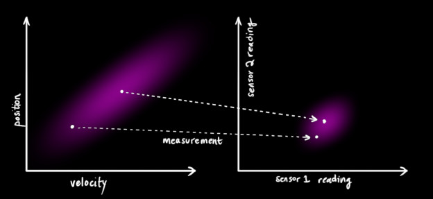
注意,传感器读取的数据的单位和尺度有可能与我们要跟踪的状态的单位和尺度不一样,我们用矩阵 来表示传感器的数据。

我们可以计算出传感器读数的分布,用之前的表示方法如下式所示:

卡尔曼滤波的一大优点就是能处理传感器噪声,换句话说,我们的传感器或多或少都有点不可靠,并且原始估计中的每个状态可以和一定范围内的传感器读数对应起来。

从测量到的传感器数据中,我们大致能猜到系统当前处于什么状态。但是由于存在不确定性,某些状态可能比我们得到的读数更接近真实状态。

我们将这种不确定性(例如:传感器噪声)用协方差

现在我们有了两个高斯分布,一个是在预测值附近,一个是在传感器读数附近。

我们必须在预测值(粉红色)和传感器测量值(绿色)之间找到最优解。
那么,我们最有可能的状态是什么呢?对于任何可能的读数

剩下的就是重叠部分了,这个重叠部分的均值就是两个估计最可能的值,也就是给定的所有信息中的最优估计。
瞧!这个重叠的区域看起来像另一个高斯分布。

如你所见,把两个具有不同均值和方差的高斯分布相乘,你会得到一个新的具有独立均值和方差的高斯分布!下面用公式讲解。
融合高斯分布
先以一维高斯分布来分析比较简单点,具有方差 和 μ 的高斯曲线可以用下式表示:

如果把两个服从高斯分布的函数相乘会得到什么呢?
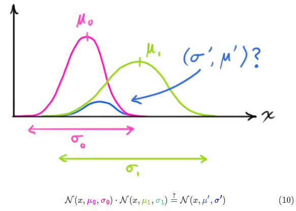
将式(9)代入到式(10)中(注意重新归一化,使总概率为1)可以得到:

将式(11)中的两个式子相同的部分用 k 表示:

下面进一步将式(12)和(13)写成矩阵的形式,如果 Σ 表示高斯分布的协方差, 表示每个维度的均值,则:

矩阵
将所有公式整合起来
我们有两个高斯分布,预测部分


由式(14)可得卡尔曼增益为:

将式(16)和式(17)的两边同时左乘矩阵的逆(注意
)将其约掉,再将式(16)的第二个等式两边同时右乘矩阵
的逆得到以下等式:

上式给出了完整的更新步骤方程。

总结
以上所有公式中,你只需要用到式(7)、(18)、(19)。(如果忘了的话,你可以根据式(4)和(15)重新推导一下)
我们可以用这些公式对任何线性系统建立精确的模型,对于非线性系统来说,我们使用扩展卡尔曼滤波,区别在于EKF多了一个把预测和测量部分进行线性化的过程。
(ps: 第一次用Markdown,添加图片和公式心累啊,什么时候能直接拖拽就好了~~)
附Markdown使用技巧:
1. 改变文本字体、字号与颜色。参考链接:(http://blog.csdn.net/testcs_dn/article/details/45719357/)
2. 在线公式编辑器,编辑好了右键“复制图片地址”,当作图片来添加。
链接:(http://private.codecogs.com/latex/eqneditor.php)
3. 段落首行缩进,按Shift+Space将输入法切换到全角状态,然后敲空格即可,一个空格代表一个汉字的间隔。
4. 设置图片大小及居中显示。参考链接:(http://blog.csdn.net/soindy/article/details/50427079)
5. 不懂百度。


【推荐】国内首个AI IDE,深度理解中文开发场景,立即下载体验Trae
【推荐】编程新体验,更懂你的AI,立即体验豆包MarsCode编程助手
【推荐】抖音旗下AI助手豆包,你的智能百科全书,全免费不限次数
【推荐】轻量又高性能的 SSH 工具 IShell:AI 加持,快人一步
· 开发者必知的日志记录最佳实践
· SQL Server 2025 AI相关能力初探
· Linux系列:如何用 C#调用 C方法造成内存泄露
· AI与.NET技术实操系列(二):开始使用ML.NET
· 记一次.NET内存居高不下排查解决与启示
· 阿里最新开源QwQ-32B,效果媲美deepseek-r1满血版,部署成本又又又降低了!
· 开源Multi-agent AI智能体框架aevatar.ai,欢迎大家贡献代码
· Manus重磅发布:全球首款通用AI代理技术深度解析与实战指南
· 被坑几百块钱后,我竟然真的恢复了删除的微信聊天记录!
· AI技术革命,工作效率10个最佳AI工具
2020-12-29 用C实现面向对象