LiMaosen-2022-SkeletonPartedGraphScattering-ECCV
Skeleton-Parted Graph Scattering Networks for 3D Human Motion Prediction #paper
1. paper-info
1.1 Metadata
- Author:: [[Maosen Li]], [[Siheng Chen]], [[Zijing Zhang]], [[Lingxi Xie]], [[Qi Tian]], [[Ya Zhang]]
- 作者机构:: 南京大学
- Keywords:: #GCN , #DCT
- Journal:: #ECCV
- Date:: [[2022-07-31]]
- 状态:: #Done
- 链接:: http://arxiv.org/abs/2208.00368
- 阅读时间:: 2023.01.04
1.2.Abstract
Graph convolutional network based methods that model the body-joints' relations, have recently shown great promise in 3D skeleton-based human motion prediction. However, these methods have two critical issues: first, deep graph convolutions filter features within only limited graph spectrums, losing sufficient information in the full band; second, using a single graph to model the whole body underestimates the diverse patterns on various body-parts. To address the first issue, we propose adaptive graph scattering, which leverages multiple trainable band-pass graph filters to decompose pose features into richer graph spectrum bands. To address the second issue, body-parts are modeled separately to learn diverse dynamics, which enables finer feature extraction along the spatial dimensions. Integrating the above two designs, we propose a novel skeleton-parted graph scattering network (SPGSN). The cores of the model are cascaded multi-part graph scattering blocks (MPGSBs), building adaptive graph scattering on diverse body-parts, as well as fusing the decomposed features based on the inferred spectrum importance and body-part interactions. Extensive experiments have shown that SPGSN outperforms state-of-the-art methods by remarkable margins of 13.8%, 9.3% and 2.7% in terms of 3D mean per joint position error (MPJPE) on Human3.6M, CMU Mocap and 3DPW datasets, respectively.
关键词:GCN,HMP,DCT
2. Introduction
- 领域:: 3D skeleton-based human motion prediction
- 之前的方法::
- state model to capture the shallow dynamics
- deep learning area:
- RNN-based
- GCN-based
- 作者主要是针对GCN-based方法。
- 问题::
- 给定图结构后,标准的图卷积只能在有限的的图谱内过滤特征,而不能显著得保留更丰富的波段。(感觉类似于生成模型的模式坍塌问题,只能集中于主要的特征,而忽略了其他边缘特征。)
- 现存的方法都用单一的图去对整个身体结构进行建模,不能够学习到身体结构之间的多模态。(就是将身体拆分,分开学习,学习到更多的模式。)
- 解决办法::
- 提出了一种自适应图散射技术(adaptive graph scattering technique):: 一种树形结构的波段图过滤器,能够将特征解构到多种图波段。主要包括三种技术(1. 基于数学的特殊波段过滤;2. 自适应过滤参数; 3.特征过滤层 )
- 将人体结构分层。
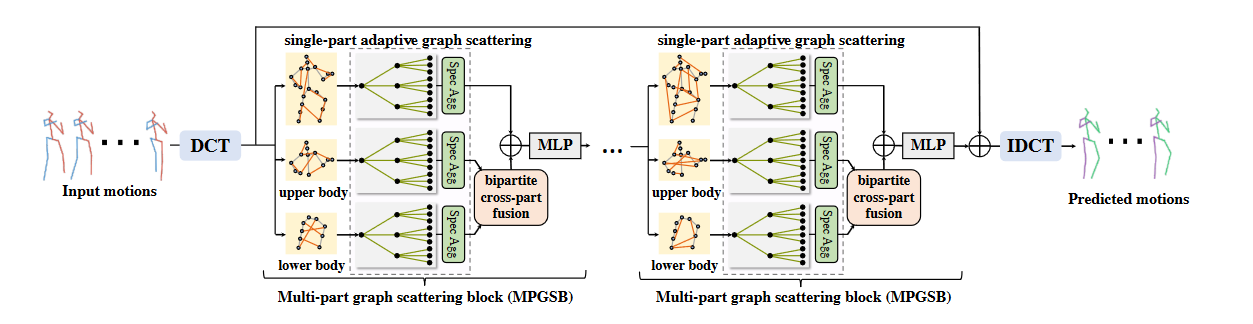
- 模型主要结构,如Fig1
- skeleton-parted graph scattering network(SPGSN):: 将人体结构分层,进行特征波段筛选。
- multi-part graph scattering block(MPGSB):: 进行波段过滤。由二部分构成,
- single-part adaptive graph scattering:: 用MPGSB去概括部分身体部分的特征。
- bipartite cross-part fusion:: 用于概括不同身体部分的特征。
- 问题::
3. Skeleton-Part Graph Scattering Network
符号描述::
\(X^{(t)}\in \mathbb{R}^{M\times 3}\):: t时刻的动作。
\(\mathbb{X} = [X_{(1)},...,X^{(T)}]\):: 动作序列
\(\mathbb{X}^-\)::历史序列
\(\mathbb{X}^+\)::预测序列
3.1 模型结构
模型如Fig.1
输入历史序列\(\mathbb{X}^-\in\mathbb{R}^{T\times M \times 3}\),首先将\(\mathbb{X}\)reshape成\(\mathcal{X}^-\in\mathbb{R}^{T\times 3M}\),目的是将每个时间戳的所有关节坐标独立地作为空间域的独立单位;然后通过DCT,\(X^{-}= DCT(\mathcal{X}^-)\in\mathbb{R}^{M' \times 3}\)其中\(M' = 3M\) ,然后通过多个multi-part graph scattering blocks(MPGSBs),同时这里使用了类似残差连接的方式,目的是让SPGSN捕获特征位移以进行稳定预测;最后通过IDCT转换为时间序列信息。
4.multi-part graph scattering blocks(MPGSB)
每个MPGSB块由两部分构成::
- single-part adaptive graph scattering:: 特征提取,学习身体部位的大波段信息。
- bipartite cross-part fusion:: 特征融合
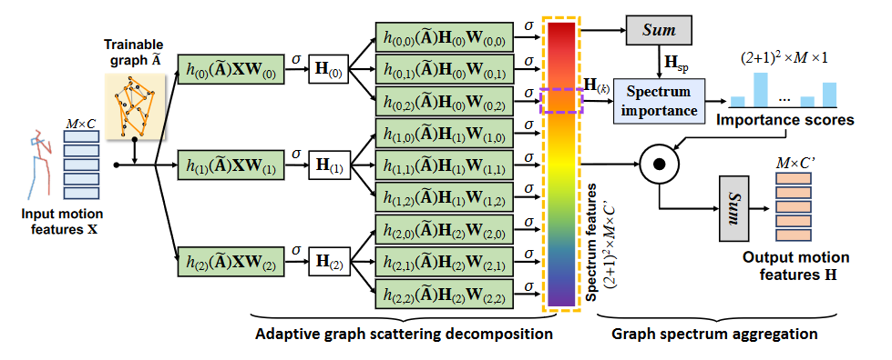
4.1 single-part adaptive graph scattering
该部分由两部分构成::
- adaptive graph scattering decomposition
- adaptive graph spectrum aggregation
adaptive graph scattering decomposition
一个树形结构的网络,\(L\)层,树的结点层指数增长。以一层说明::
输入DCT-formed pose feature\(X\in\mathbb{R}^{M'\times C}\) 和 对应的领接矩阵\(A\in\mathbb{R}^{M'\times M'}\),然后通过一系列的带通图形滤波器(bandpass graph filters)\(\{ h_{(k)}(\tilde{A} )| k=0,1,...,K \}\) ,其中 \(\tilde{A}=\tilde{A} = 1/2(I+A/\left \| A \right \|_F^2 )\),归一化;通过这些filter bank,得到特征::
其中\(W_{(k)}\)是可学习的参数,\(\sigma(.)\)用于分散图形频率表示,也就是激活函数。
为了能够让filter作用不同的图波段,通过数学先验对他进行初始化,然后通过可学习的系数对filter进行微调,计算方式如下::
其中\(\alpha_{(k,j)}\)为可学习的系数。当\(k=0\)时,\(\alpha_{(0,0)}=1\),当\(k>0\)时,\(\alpha_{(k,k-1)=1}, \ \alpha_{(k,k)}=-1\),其他的\(\alpha_{(k,j)}=0\)。
重复上面的过程,每一层都得到\(K+1\)个分支,最后经过\(L\)层后,就会得到\((K+1)^L\)个channels,对应不同的波段。
adaptive graph spectrum aggregation
对不同波段的信息进行筛选融合,也就是特征筛选,通过对不同的波段特征加入可学习的参数,计算方式如下::
\(\mathcal{w}_k\)就是频谱重要性分数系数,计算方式如下::
其中\(f_1(.) \ and \ f_2(.)\)为全连接层,\([.,.]\)为沿着特征维度串联,\(H_{sp}\in\mathbb{R}^{M'\times C'}\)的计算方式::
例子
\(L=2 \ K=2\)
4.2 Bipartite Cross-Part Fusion
对不同身体部分的特征进行选择融合。在本paper中,作者将人体结构分为上下两部分。
输入\(H_{\uparrow}\in\mathbb{R}^{M_\uparrow \times C'}\)上半部分的特征,\(H_{\downarrow }\in\mathbb{R}^{M_\downarrow \times C'}\)下班部分特征,首先得到upper-to-lower affinity matrix::
\(f_{\uparrow}(.) \ and \ f_{\downarrow}(.)\)为两个编码网络。
得到映射矩阵后,更新两部分的特征通过下面的公式::
最后,将整个身体的特征于部分混合特征融合,通过下面的公式得到\(H'\in\mathbb{R}^{M'\times C'}\)
\(\oplus: \mathbb{R}^{M_{\uparrow} \times C^{\prime}} \times \mathbb{R}^{M_{\downarrow} \times C^{\prime}} \rightarrow \mathbb{R}^{M^{\prime} \times C^{\prime}}\)放置来自不同身体部位的关节以与原始身体对齐。
4.3 Loss function
重构损失::
5. Experiments
- dataset
- Human 3.6M
- CMU Mocap
- 3D pose in the wild(3DPW)
6. 代码
DCT 实现
def get_dct_matrix(N):
    dct_m = np.eye(N)
    for k in np.arange(N):
        for i in np.arange(N):
            w = np.sqrt(2 / N)
            if k == 0:
                w = np.sqrt(1 / N)
            dct_m[k, i] = w * np.cos(np.pi * (i + 1 / 2) * k / N)
    idct_m = np.linalg.inv(dct_m)
    return dct_m, idct_m
7. 总结
总得来说就是针对模型学习会集中到低频率的特征,而忽略高频段的特征,于是将特征解构。

 浙公网安备 33010602011771号