003-simonyanVeryDeepConvolutional2015(VGG)
Very Deep Convolutional Networks for Large-Scale Image Recognition #paper
1. paper-info
1.1 Metadata
- Author::[[Karen Simonyan]], [[Andrew Zisserman]]
- 作者机构::
- Keywords:: #DeepLearning , #VGG, #CNN
- Journal:: [[2015-04-10]]
- 状态:: #Doing
1.2 Abstract
In this work we investigate the effect of the convolutional network depth on its accuracy in the large-scale image recognition setting. Our main contribution is a thorough evaluation of networks of increasing depth using an architecture with very small (3 × 3) convolution filters, which shows that a significant improvement on the prior-art configurations can be achieved by pushing the depth to 16–19 weight layers. These findings were the basis of our ImageNet Challenge 2014 submission, where our team secured the first and the second places in the localisation and classification tracks respectively. We also show that our representations generalise well to other datasets, where they achieve state-of-the-art results. We have made our two best-performing ConvNet models publicly available to facilitate further research on the use of deep visual representations in computer vision.
2. The Architecture
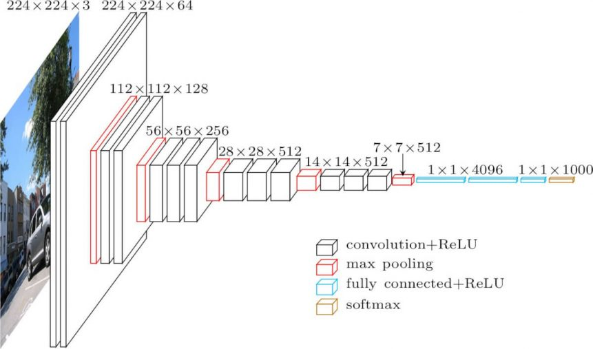
2.1 网络输入
在训练过程中,网络输入尺寸固定为 224×224 的 RGB 图像,唯一的预处理就是:基于整个训练集计算 RGB 的均值,然后每个像素节点上减去该均值。
2.2 网络各层结构
- 卷积层:在这里,网络用
3×3的小尺寸卷积核来提取特征,并用1×1的卷积核来作线性转换(后接非线性层)。卷积运算的步长设置为1,且进行padding,使得卷积前后尺寸不变。 - 激活函数: ReLU,由于
Local Response Normalisation (LRN)对网络无益,所以网络未使用。 - 池化层:池化层选取
max-pooling,步长为2, 尺寸为2 * 2。 因此,特征图的尺寸变换只发生于池化层。 - 全连接层:网络最后,接着
3个全连接层(Fully-Connected layers)。神经元数目分别为:4096,4096,1000,最后1000用于1000分类。最后用一个softmax层,用于计算类别的概率(约束在0~1之间,和为1)。
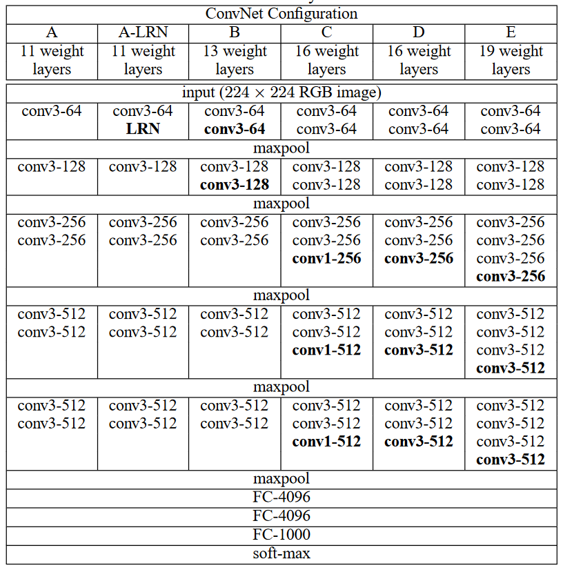
2.3 CONFIGURATIONS
本文验证了多种 VGG 结构,各个结构只有深度不同,其余配置一样。分别用 A-E 表示,如图2-2;conv3-64: 64个(3x3)卷积核

3. CLASSIFICATION FRAMEWORK
3.1 超参数配置
模型训练使用小批量随机梯度下降进行优化,且 momentum = 0.9。训练过程中使用 weight decay 进行正则化,其中,L2 衰减因子设为 \(5e-4\)。在全连接层的前两层,使用了 [[dropout]],系数为 0.5。
学习速率初始化为 0.01,每次且当验证集精度不再改善时,将其减少到 1/10 。在我们的训练中,一共衰减 3 次,最后在 370K 次迭代(74 epoch)时,停止训练。
3.2 模型参数初始化
网络参数初始化极其重要,因为不好的初始化可能导致模型停滞于不稳定的梯度。所以,我们先用 A 模型进行训练,对于 A 用随机初始化。然后其后的网络类型(B-E)的初始化中,其前四层以及最后的 3 层全连接层,用 A 的参数进行初始化,其余层进行随机初始化。并且,未减小学习速率。
对于随机初始化,本文随机采样 0 均值,0.01 方差的正态分布作为权值,bias 则初始化为 0。
3.3 图片训练尺寸
设训练图像(宽长相等)的最小尺寸为 S,在图像输入时,还需要进行 crop 以及其他预处理(见下面的输入图像处理)。本文是用了两种方式来设置 S。
-
第一种是,使用固定尺寸的
S,这样通过crop仍能实现multi-scale。本文尝试了256和384两种尺寸。首先使用256的尺寸进行训练。然后直接将其作为384的初始参数,并将学习速率调低至0.001。 -
第二种是设置
S在一个范围内。每次训练时,每张图像被随机rescaled到 1/10 中的一个值。可以将这种方式视为一种数据增强。为了加快训练,使用前面固定尺寸384训练出来的模型参数作为初始化。
4. Testing
5. CLASSIFICATION EXPERIMENTS
5.1 SINGLE SCALE EVALUATION
用单一尺度对每个模型(共6个,模型参数如图 2-2)进行评估。评估结果如图 5-1,
测试图像尺寸依训练时的尺寸设定分为两种情况:
- 训练图像的尺寸S固定时,设置训练图像尺寸S等于测试图像尺寸Q;
- 训练图像尺寸S是介于[Smin,Smax]时,设置测试图像尺寸Q=0.5(Smin+Smax)。
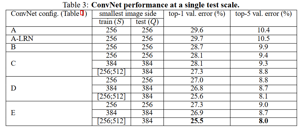
实验结果:
- 运用LRN的模型并没有提高模型的准确率。
- 网络深度增加,网络的性能也增加。
- conv1x1的非线性变化有作用(C和D)。C和D网络层数相同,但D将C的3个conv3x3换成了conv1x1,性能提升。这点我理解是,跨通道的信息交换/融合,可以产生丰富的特征易于分类器学习。conv1x1相比conv3x3不会去学习local的局部像素信息,专注于跨通道的信息交换/融合,同时为后面全连接层(全连接层相当于global卷积)做准备,使之学习过程更自然。
- 多小卷积核比单大卷积核性能好(B)。作者做了实验用B和自己一个不在实验组里的较浅网络比较,较浅网络用conv5x5来代替B的两个conv3x3。多个小卷积核比单大卷积核效果好,换句话说当考虑卷积核大小时:depths matters。
5.2 MULTI-SCALE EVALUATION
也就是对输入图像在一定范围内的随机尺度缩放,模型最终的结果,是基于不同尺度(赌赢多个不同值的Q)且是crop后的图像跑网络得到的softmax结果的平均。
- 用固定大小的尺度S训练的模型,用三种尺寸Q去评估,其中Q=[S–32,S,S+32] ;
- 用尺度S随机的方式训练模型,S∈[Smin;Smax],评估使用更大的尺寸范围Q={Smin,0.5(Smin+Smax),Smax}
评估结果如图5-2


6. 代码实现(pytorch)
6.1 加载数据
Dataset
数据集 CIFAR-100
该数据集有100个分类,20大类。

导包
import numpy as np
import torch
import torch.nn as nn
from torchvision import datasets
from torchvision import transforms
from torch.utils.data.sampler import SubsetRandomSampler
device = torch.device('cuda' if torch.cuda.is_available() else 'cpu')
- np: 数学操作。
- torch: 构建模型结构。
- torchvision:用于数据加载/处理,包含数据集和在计算机视觉中处理这些数据集的方法。
加载数据
def data_loader(data_dir,
                batch_size,
                random_seed=42,
                valid_size=0.1,
                shuffle=True,
                test=False):

    normalize = transforms.Normalize(
        mean=[0.4914, 0.4822, 0.4465],
        std=[0.2023, 0.1994, 0.2010],
    )

    # define transforms
    transform = transforms.Compose([
            transforms.Resize((227,227)),
            transforms.ToTensor(),
            normalize,
    ])

    if test:
        dataset = datasets.CIFAR100(
          root=data_dir, train=False,
          download=True, transform=transform,
        )

        data_loader = torch.utils.data.DataLoader(
            dataset, batch_size=batch_size, shuffle=shuffle
        )

        return data_loader

    # load the dataset
    train_dataset = datasets.CIFAR100(
        root=data_dir, train=True,
        download=True, transform=transform,
    )

    valid_dataset = datasets.CIFAR10(
        root=data_dir, train=True,
        download=True, transform=transform,
    )

    num_train = len(train_dataset)
    indices = list(range(num_train))
    split = int(np.floor(valid_size * num_train))

    if shuffle:
        np.random.seed(random_seed)
        np.random.shuffle(indices)

    train_idx, valid_idx = indices[split:], indices[:split]
    train_sampler = SubsetRandomSampler(train_idx)
    valid_sampler = SubsetRandomSampler(valid_idx)

    train_loader = torch.utils.data.DataLoader(
        train_dataset, batch_size=batch_size, sampler=train_sampler)

    valid_loader = torch.utils.data.DataLoader(
        valid_dataset, batch_size=batch_size, sampler=valid_sampler)

    return (train_loader, valid_loader)


## CIFAR100 dataset
train_loader, valid_loader = data_loader(data_dir='./data',
                                         batch_size=64)

test_loader = data_loader(data_dir='./data',
                              batch_size=64,
                              test=True)
6.2 构建VGG16模型
class VGG16(nn.Module):
    def __init__(self, num_classes=10):
        super(VGG16, self).__init__()
        self.layer1 = nn.Sequential(
            nn.Conv2d(3, 64, kernel_size=3, stride=1, padding=1),
            nn.BatchNorm2d(64),
            nn.ReLU())
        self.layer2 = nn.Sequential(
            nn.Conv2d(64, 64, kernel_size=3, stride=1, padding=1),
            nn.BatchNorm2d(64),
            nn.ReLU(),
            nn.MaxPool2d(kernel_size = 2, stride = 2))
        self.layer3 = nn.Sequential(
            nn.Conv2d(64, 128, kernel_size=3, stride=1, padding=1),
            nn.BatchNorm2d(128),
            nn.ReLU())
        self.layer4 = nn.Sequential(
            nn.Conv2d(128, 128, kernel_size=3, stride=1, padding=1),
            nn.BatchNorm2d(128),
            nn.ReLU(),
            nn.MaxPool2d(kernel_size = 2, stride = 2))
        self.layer5 = nn.Sequential(
            nn.Conv2d(128, 256, kernel_size=3, stride=1, padding=1),
            nn.BatchNorm2d(256),
            nn.ReLU())
        self.layer6 = nn.Sequential(
            nn.Conv2d(256, 256, kernel_size=3, stride=1, padding=1),
            nn.BatchNorm2d(256),
            nn.ReLU())
        self.layer7 = nn.Sequential(
            nn.Conv2d(256, 256, kernel_size=3, stride=1, padding=1),
            nn.BatchNorm2d(256),
            nn.ReLU(),
            nn.MaxPool2d(kernel_size = 2, stride = 2))
        self.layer8 = nn.Sequential(
            nn.Conv2d(256, 512, kernel_size=3, stride=1, padding=1),
            nn.BatchNorm2d(512),
            nn.ReLU())
        self.layer9 = nn.Sequential(
            nn.Conv2d(512, 512, kernel_size=3, stride=1, padding=1),
            nn.BatchNorm2d(512),
            nn.ReLU())
        self.layer10 = nn.Sequential(
            nn.Conv2d(512, 512, kernel_size=3, stride=1, padding=1),
            nn.BatchNorm2d(512),
            nn.ReLU(),
            nn.MaxPool2d(kernel_size = 2, stride = 2))
        self.layer11 = nn.Sequential(
            nn.Conv2d(512, 512, kernel_size=3, stride=1, padding=1),
            nn.BatchNorm2d(512),
            nn.ReLU())
        self.layer12 = nn.Sequential(
            nn.Conv2d(512, 512, kernel_size=3, stride=1, padding=1),
            nn.BatchNorm2d(512),
            nn.ReLU())
        self.layer13 = nn.Sequential(
            nn.Conv2d(512, 512, kernel_size=3, stride=1, padding=1),
            nn.BatchNorm2d(512),
            nn.ReLU(),
            nn.MaxPool2d(kernel_size = 2, stride = 2))
        self.fc = nn.Sequential(
            nn.Dropout(0.5),
            nn.Linear(7*7*512, 4096),
            nn.ReLU())
        self.fc1 = nn.Sequential(
            nn.Dropout(0.5),
            nn.Linear(4096, 4096),
            nn.ReLU())
        self.fc2= nn.Sequential(
            nn.Linear(4096, num_classes))

    def forward(self, x):
        out = self.layer1(x)
        out = self.layer2(out)
        out = self.layer3(out)
        out = self.layer4(out)
        out = self.layer5(out)
        out = self.layer6(out)
        out = self.layer7(out)
        out = self.layer8(out)
        out = self.layer9(out)
        out = self.layer10(out)
        out = self.layer11(out)
        out = self.layer12(out)
        out = self.layer13(out)
        out = out.reshape(out.size(0), -1)
        out = self.fc(out)
        out = self.fc1(out)
        out = self.fc2(out)
        return out
6.3 设置超参数
num_classes = 100
num_epochs = 20
batch_size = 16
learning_rate = 0.005

model = VGG16(num_classes).to(device)


# Loss and optimizer
criterion = nn.CrossEntropyLoss()
optimizer = torch.optim.SGD(model.parameters(), lr=learning_rate, weight_decay = 0.005, momentum = 0.9)


# Train the model
total_step = len(train_loader)
6.4 训练
total_step = len(train_loader)

for epoch in range(num_epochs):
    for i, (images, labels) in enumerate(train_loader):
        # Move tensors to the configured device
        images = images.to(device)
        labels = labels.to(device)

        # Forward pass
        outputs = model(images)
        loss = criterion(outputs, labels)

        # Backward and optimize
        optimizer.zero_grad()
        loss.backward()
        optimizer.step()

    print ('Epoch [{}/{}], Step [{}/{}], Loss: {:.4f}'
                   .format(epoch+1, num_epochs, i+1, total_step, loss.item()))

    # Validation
    with torch.no_grad():
        correct = 0
        total = 0
        for images, labels in valid_loader:
            images = images.to(device)
            labels = labels.to(device)
            outputs = model(images)
            _, predicted = torch.max(outputs.data, 1)
            total += labels.size(0)
            correct += (predicted == labels).sum().item()
            del images, labels, outputs

        print('Accuracy of the network on the {} validation images: {} %'.format(5000, 100 * correct / total))
训练过程较久,耐心等待。
6.5 测试
with torch.no_grad():
    correct = 0
    total = 0
    for images, labels in test_loader:
        images = images.to(device)
        labels = labels.to(device)
        outputs = model(images)
        _, predicted = torch.max(outputs.data, 1)
        total += labels.size(0)
        correct += (predicted == labels).sum().item()
        del images, labels, outputs

    print('Accuracy of the network on the {} test images: {} %'.format(10000, 100 * correct / total))
7. 总结 #summary
- 很多东西都是参考别人的理解得到,自主理解较浅。
- 3x3卷积核能够使得网络更深,原因在于3x3卷积核叠加之后也能够获得大卷积核的
感受野,并且小卷积核所需要的参数更少,有利于性能提升。 - 训练和预测时的技巧,训练时先训练级别A的简单网络,再复用A网络的权重来初始化后面的几个复杂模型,这样训练收敛的速度更快。预测时采用Multi-Scale的方法,同时还再训练时VGGNet也使用了Multi-Scale的方法做数据增强。
参考
https://distill.pub/2017/feature-visualization/ feature-visualization
http://www.robots.ox.ac.uk/~karen/pdf/ILSVRC_2014.pdf ILSVRC-2014 presentation
http://cs231n.stanford.edu/slides/2017/cs231n_2017_lecture9.pdf
https://machinethink.net/blog/convolutional-neural-networks-on-the-iphone-with-vggnet/ Convolutional neural networks on the iPhone with VGGNet
https://www.aiuai.cn/aifarm138.html VGG模型详解
https://blog.paperspace.com/vgg-from-scratch-pytorch/ Writing VGG from Scratch in PyTorch
Zotero links
-
- Cite key: simonyanVeryDeepConvolutional2015

 浙公网安备 33010602011771号