TensorFlow学习笔记

TensorFlow

Course 1 and Course 2

【吴恩达团队Tensorflow2.0实践系列课程第一课】TensorFlow2.0中基于TensorFlow2.0的人工智能、机器学习和深度学习简介及基础编程

【吴恩达团队Tensorflow2.0实践系列课程第二课】卷积神经网络在TensorFlow2.0中的应用_哔哩哔哩_bilibili

1. Download files with Python

from requests import get
from time import time
from math import floor
from tqdm import tqdm

url = '...'
file_name = '...'

with get(url, stream=True) as r:
    print("正在检查资源大小")
    b = int(r.headers.get('Content-Length')) / 1024 / 1024
    print("资源大小：", b, "MB")
    print('-' * 32)
    chunk_size = 1048
    print("正在下载")

    a = time()
    with open('./tmp/' + file_name, "wb") as code:
        for chunk in tqdm(r.iter_content(chunk_size=chunk_size)):
            code.write(chunk)
            code.flush()
        code.close()
    '''
    with open('./tmp/' + file_name, "wb") as f:
        f.write(r.content)
        f.flush()
        f.close()
    '''
    a = time() - a
    if a :
        print("平均写入速度：约", floor((b / a) * 100) / 100, "MB/s")
    else:
        print("平均写入速度：约 0 MB/s")
    print('-' * 32)

2. Unzip the zip file with Python

import zipfile

local_zip = './tmp/horse-or-human.zip'
zip_ref = zipfile.ZipFile(local_zip, 'r')
zip_ref.extractall('./tmp/horse-or-human')
local_zip = './tmp/validation-horse-or-human.zip'
zip_ref = zipfile.ZipFile(local_zip, 'r')
zip_ref.extractall('./tmp/validation-horse-or-human')
zip_ref.close()

3. Show data sample images

import matplotlib.pyplot as plt
import matplotlib.image as mpimg

nrows = 4
ncols = 4
pic_index = 0

fig = plt.gcf()
fig.set_size_inches(ncols * 4, nrows * 4)

pic_index += 8
next_horse_pix = [os.path.join(train_horse_dir, fname)
                  for fname in train_horse_names[pic_index - 8:pic_index]]
next_human_pix = [os.path.join(train_human_dir, fname)
                  for fname in train_human_names[pic_index - 8:pic_index]]

for i, img_path in enumerate(next_horse_pix + next_human_pix):
    sp = plt.subplot(nrows, ncols, i + 1)
    sp.axis('Off')

    img = mpimg.imread(img_path)
    plt.imshow(img)

plt.show()

4. ImageDataGenerator and Image augmentation

参数解释：

• rotation_range is a value in degrees (0–180), a range within which to randomly rotate pictures.
• width_shift and height_shift are ranges (as a fraction of total width or height) within which to randomly translate pictures vertically or horizontally.
• shear_range is for randomly applying shearing transformations.
• zoom_range is for randomly zooming inside pictures.
• horizontal_flip is for randomly flipping half of the images horizontally. This is relevant when there are no assumptions of horizontal assymmetry (e.g. real-world pictures).
• vertical_flip
• fill_mode is the strategy used for filling in newly created pixels, which can appear after a rotation or a width/height shift.
• validation_split=0.2 and subset='validation'

from keras.preprocessing.image import ImageDataGenerator

train_datagen = ImageDataGenerator(
    rescale=1/255,
    rotation_range=40,
    width_shift_range=0.2,
    height_shift_range=0.2,
    shear_range=0.2,
    zoom_range=0.2,
    horizontal_flip=True,
    fill_mode='nearest'
)
validation_datagen = ImageDataGenerator(rescale=1/255)

train_generator = train_datagen.flow_from_directory(
    './tmp/horse-or-human/',
    target_size=(300, 300),
    batch_size=32,
    class_mode='binary'
)
validation_generator = validation_datagen.flow_from_directory(
    './tmp/validation-horse-or-human/',
    target_size=(300, 300),
    batch_size=32,
    class_mode='binary'
)

5. Building and running the model

import tensorflow as tf

model = tf.keras.models.Sequential([
    tf.keras.layers.Conv2D(16, (3, 3), activation='relu', input_shape=(300, 300, 3)),
    tf.keras.layers.MaxPooling2D(2, 2),
    tf.keras.layers.Conv2D(32, (3, 3), activation='relu'),
    tf.keras.layers.MaxPooling2D(2, 2),
    tf.keras.layers.Conv2D(64, (3, 3), activation='relu'),
    tf.keras.layers.MaxPooling2D(2, 2),
    tf.keras.layers.Conv2D(64, (3, 3), activation='relu'),
    tf.keras.layers.MaxPooling2D(2, 2),
    tf.keras.layers.Conv2D(64, (3, 3), activation='relu'),
    tf.keras.layers.MaxPooling2D(2, 2),

    tf.keras.layers.Flatten(),
    tf.keras.layers.Dropout(0.5),
    tf.keras.layers.Dense(512, activation='relu'),
    tf.keras.layers.Dense(1, activation='sigmoid')
])

model.summary()

model.compile(loss='binary_crossentropy',
              optimizer=tf.keras.optimizers.RMSprop(0.001),
              metrics=['acc'])

history = model.fit(
    train_generator,
    steps_per_epoch=32,
    epochs=15,
    verbose=1,
    validation_data=validation_generator,
    validation_steps=8
)

6. Evaluating the model

import matplotlib.pyplot as plt

acc = history.history['acc']
val_acc = history.history['val_acc']
loss = history.history['loss']
val_loss = history.history['val_loss']

epochs = range(len(acc))

plt.figure()
plt.plot(epochs, acc, 'bo', label='Training accuracy')
plt.plot(epochs, val_acc, 'b', label='Validation accuracy')
plt.title('Training and validation accuracy')

plt.figure()
plt.plot(epochs, loss, 'bo', label='Training Loss')
plt.plot(epochs, val_loss, 'b', label='Validation Loss')
plt.title("Training and validation loss")
plt.legend()

plt.show()

7. Predicting

import numpy as np
from keras.utils import image_utils
from tkinter.filedialog import askopenfilename

path_img = askopenfilename()
img = image_utils.load_img(path_img, target_size=(300, 300))
x = image_utils.img_to_array(img)
x = np.expand_dims(x, axis=0)
print(x.shape)
images = np.vstack([x])
print(images.shape)
classes = model.predict(images, batch_size=10)
print(classes)
if classes[0] > 0.5:
    print("It is a human")
else:
    print("It is a horse")

import numpy as np
import os
from keras.preprocessing.image import load_img, img_to_array

test_dir = './test1/'
test_id = os.listdir(test_dir)

alls = []
for f in test_id:
    image = load_img(os.path.join(test_dir, f), target_size=(150, 150))
    x = img_to_array(image)
    x = np.expand_dims(x, axis=0)
    alls.append(x)
images = np.vstack(alls)    
print(images.shape)
predictions = model.predict(images).flatten().astype(int)

8. Visualizing intermediate representations

import numpy as np
import random
from keras.utils.image_utils import load_img, img_to_array

successive_outputs = [layer.output for layer in model.layers[1:]]
visualization_model = tf.keras.models.Model(inputs=model.input, outputs=successive_outputs)

horse_img_files = [os.path.join(train_horse_dir, f) for f in train_horse_names]
human_img_files = [os.path.join(train_human_dir, f) for f in train_human_names]
img_path = random.choice(horse_img_files + human_img_files)

img = load_img(img_path, target_size=(300, 300))
x = img_to_array(img)
x = x.reshape((1, ) + x.shape)
x /= 255

successive_feature_maps = visualization_model.predict(x)
layer_names = [layer.name for layer in model.layers]

for layer_name, feature_map in zip(layer_names, successive_feature_maps):
    if len(feature_map.shape) == 4:
        n_features = feature_map.shape[-1]
        size = feature_map.shape[1]
        display_grid = np.zeros((size, size * n_features))
        for i in range(n_features):
            x = feature_map[0, :, :, i]
            x -= x.mean()
            x /= x.std()
            x *= 64
            x += 128
            x = np.clip(x, 0, 255).astype('uint8')
            display_grid[:, i * size : (i + 1) * size] = x
        scale = 20. / n_features
        plt.figure(figsize=(scale * n_features, scale))
        plt.title(layer_name)
        plt.grid(False)
        plt.imshow(display_grid, aspect='auto', cmap='viridis')

layer_outputs = [layer.output for layer in model.layers]
activation_model = tf.keras.models.Model(inputs=model.input, outputs=layer_outputs)

print(test_labels[:100])
for x in range(0, 4):
    f1 = activation_model.predict(test_images[FIRST_IMAGE].reshape(1, 28, 28, 1))[x]
    axarr[0, x].imshow(f1[0, :, :, CONVOLUTION_NUMBER], cmap='inferno')
    axarr[0, x].grid(False)
    f2 = activation_model.predict(test_images[SECOND_IMAGE].reshape(1, 28, 28, 1))[x]
    axarr[1, x].imshow(f2[0, :, :, CONVOLUTION_NUMBER], cmap='inferno')
    axarr[1, x].grid(False)
    f3 = activation_model.predict(test_images[THIRD_IMAGE].reshape(1, 28, 28, 1))[x]
    axarr[2, x].imshow(f3[0, :, :, CONVOLUTION_NUMBER], cmap='inferno')
    axarr[2, x].grid(False)
plt.show()

9. Callbacks

import tensorflow as tf


class myCallback(tf.keras.callbacks.Callback):
    def on_epoch_end(self, epoch, log={}):
        if log.get('accuracy') > 0.998:
            print("\nReached 99.8% accuracy so cancelling training!")
            self.model.stop_training = True


mnist = tf.keras.datasets.mnist

(x_train, y_train), (x_test, y_test) = mnist.load_data()
x_train = x_train.reshape(-1, 28, 28, 1)
x_test = x_test.reshape(-1, 28, 28, 1)
x_train = x_train / 255.0
x_test = x_test / 255.0

callbacks = myCallback()

model = tf.keras.models.Sequential([
    tf.keras.layers.Conv2D(64, (3, 3), activation='relu', input_shape=(28, 28, 1)),
    tf.keras.layers.MaxPooling2D(2, 2),
    tf.keras.layers.Flatten(),
    tf.keras.layers.Dense(512, activation='relu'),
    tf.keras.layers.Dense(10, activation='softmax')
])

model.compile(optimizer='adam',
              loss='sparse_categorical_crossentropy',
              metrics=['accuracy'])

model.fit(x_train, y_train, epochs=20, callbacks=[callbacks])
model.evaluate(x_test, y_test)

10. Transfer learning

from keras import layers, Model
from keras.applications.inception_v3 import InceptionV3
from keras.optimizers import RMSprop

local_weights_file = './tmp/inception_v3_weights_tf_dim_ordering_tf_kernels_notop.h5'

pre_trained_model = InceptionV3(input_shape=(150, 150, 3),
                                include_top=False,
                                weights=None)
pre_trained_model.load_weights(local_weights_file)

for layer in pre_trained_model.layers:
    layer.trainable = False

pre_trained_model.summary()

last_layer = pre_trained_model.get_layer('mixed7')
print('last layer output shape:', last_layer.output_shape)
last_output = last_layer.output

x = layers.Flatten()(last_output)
x = layers.Dense(1024, activation='relu')(x)
x = layers.Dropout(0.2)(x)
x = layers.Dense(1, activation='sigmoid')(x)

model = Model(pre_trained_model.input, x)
model.compile(optimizer=RMSprop(0.0001),
              loss='binary_crossentropy',
              metrics=['acc'])

---

Some models:

• VGG16
• InceptionV3

Course 3: Natural Language Processing in TensorFlow

【吴恩达团队Tensorflow2.0实践系列课程第三课】TensorFlow2.0中的自然语言处理

0. Dateset(json and tfds)

import json

with open('./tmp/sarcasm.json', 'r') as f:
    datastore = json.load(f)

sentences = []
labels = []
urls = []
for item in datastore:
    sentences.append(item['headline'])
    labels.append(item['is_sarcastic'])
    urls.append(item['article_link'])

'''
name: 表示数据集的名字
split: 表示数据集的分隔方式
data_dir: 表示读写数据集的目录
batch_size: 指定数据集中每一条数据的大小，默认为1。
shuffle_files: 表示是否打乱输入的数据
download:表示是否将数据集下载到本地，默认为True，如果设置为False，相当于在三个步骤中少了builder.download_and_prepare()这一步。
as_supervised: 为True表示数据集的每一条数据保存为监督学习的方式–2元组（input, label)，如果为False表示数据集的每一条数据保存为字典类型{feature1:input, feature:label}。
with_info:如果为True，表示返回的数据集为一个元组 (tf.data.Dataset, tfds.core.DatasetInfo)；如果为False，则返回为一个tf.data.Dataset对象。
'''

import tensorflow_datasets as tfds

imdb, info = tfds.load("imdb_reviews/subwords8k", data_dir='./tmp/', with_info=True, as_supervised=True)

1. Tokenizer

import tensorflow as tf
from keras.preprocessing.text import Tokenizer
from keras_preprocessing.sequence import pad_sequences

vocab_size = 10000
embedding_dim = 16
max_length = 100
trunc_type = 'post'
padding_type = 'post'
oov_tok = '<OOV>'
training_size = 20000

tokenizer = Tokenizer(num_words=vocab_size, oov_token=oov_tok)
tokenizer.fit_on_texts(training_sentence)

word_index = tokenizer.word_index
index_word = tokenizer.index_word

training_sequences = tokenizer.texts_to_sequences(training_sentence)
training_padded = pad_sequences(training_sequences,
                                maxlen=max_length,
                                padding=padding_type,
                                truncating=trunc_type)

test_sequences = tokenizer.texts_to_sequences(test_sentence)
test_padded = pad_sequences(test_sequences,
                            maxlen=max_length,
                            padding=padding_type,
                            truncating=trunc_type)

2. Embedding

# 第二层用Flatten效果更好，但耗时更长
model = tf.keras.Sequential([
    tf.keras.layers.Embedding(vocab_size, embedding_dim, input_length=max_length),
    tf.keras.layers.GlobalMaxPool1D(),
    tf.keras.layers.Dense(24, activation='relu'),
    tf.keras.layers.Dense(1, activation='sigmoid')
])

3. Decode

def decode_sentence(text):
    return ' '.join([index_word.get(i, '?') for i in text])

4. Word to Vector

Embedding projector - visualization of high-dimensional data (tensorflow.org)

import io

out_v = io.open('./tmp/vecs_1.tsv', 'w', encoding='utf-8')
out_m = io.open('./tmp/meta_1.tsv', 'w', encoding='utf-8')

for word_num in range(1, vocab_size):
    word = index_word[word_num]
    embeddings = weights[word_num]
    out_m.write(word + '\n')
    out_v.write('\t'.join([str(x) for x in embeddings]) + '\n')
out_m.close()
out_v.close()

5. RNN

model = tf.keras.Sequential([
    tf.keras.layers.Embedding(tokenizer.vocab_size, 64),
    tf.keras.layers.Bidirectional(tf.keras.layers.LSTM(64)),
    tf.keras.layers.Dense(64, activation='relu'),
    tf.keras.layers.Dense(1, activation='sigmoid')
])

model2 = tf.keras.Sequential([
    tf.keras.layers.Embedding(tokenizer.vocab_size, 64),
    tf.keras.layers.Bidirectional(tf.keras.layers.LSTM(64, return_sequences=True)),
    tf.keras.layers.Bidirectional(tf.keras.layers.LSTM(32)),
    tf.keras.layers.Dense(64, activation='relu'),
    tf.keras.layers.Dense(1, activation='sigmoid')
])

model3 = tf.keras.Sequential([
    tf.keras.layers.Embedding(tokenizer.vocab_size, 64),
    tf.keras.layers.Bidirectional(tf.keras.layers.GRU(32)),
    tf.keras.layers.Dense(6, activation='relu'),
    tf.keras.layers.Dense(1, activation='sigmoid')
])

# CNN
model4 = tf.keras.Sequential([
    tf.keras.layers.Embedding(tokenizer.vocab_size, 64),
    tf.keras.layers.Conv1D(128, 5, activation='relu'),
    tf.keras.layers.GlobalAveragePooling1D(),
    tf.keras.layers.Dense(62, activation='relu'),
    tf.keras.layers.Dense(1, activation='sigmoid')
])

6. Generate text

# 生成语料库
tokenizer = Tokenizer()

data = "In the town of Athy one Jeremy Lanigan \n Battered away til he hadnt a pound. \nHis father died and made him a man again \n ..."
corpus = data.lower().split('\n')

tokenizer.fit_on_texts(corpus)
total_words = len(tokenizer.word_index) + 1

# 生成特征与标签
input_sequences = []
for line in corpus:
    token_list = tokenizer.texts_to_sequences([line])[0]
    for i in range(1, len(token_list)):
        n_gram_sequence = token_list[:i+1]
        input_sequences.append(n_gram_sequence)

max_sequence_len = max([len(x) for x in input_sequences])
input_sequences = pad_sequences(input_sequences, maxlen=max_sequence_len, padding='pre')
# input_sequences = np.array(input_sequences)
print(type(input_sequences))

xs, labels = input_sequences[:, :-1], input_sequences[:, -1]
ys = tf.keras.utils.to_categorical(labels, num_classes=total_words)

# build and train the model
model = Sequential()
model.add(Embedding(total_words, 64, input_length=max_sequence_len-1))
model.add(Bidirectional(LSTM(20)))
model.add(Dense(total_words, activation='softmax'))
model.compile(loss='categorical_crossentropy', optimizer='adam', metrics=['accuracy'])
model.summary()
history = model.fit(xs, ys, epochs=500, verbose=1)

# generate text
seed_text = "Laurence went to dublin"
next_words = 100

for _ in range(next_words):
    token_list = tokenizer.texts_to_sequences([seed_text])[0]
    token_list = pad_sequences([token_list], maxlen=max_sequence_len-1, padding='pre')
    predict = model.predict(token_list, verbose=0)
    predict = predict.argmax()
    seed_text += ' ' + tokenizer.index_word[predict]
print(seed_text)

Course 4: Sequences, Time Series and Prediction

【吴恩达团队Tensorflow2.0实践系列课程第四课】序列、时间序列和预测_哔哩哔哩_bilibili

1. Create some time series

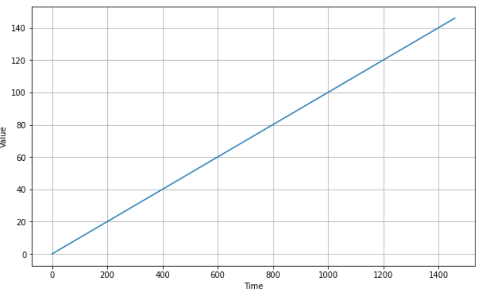
a. Trend

# trend
def trend(time, slope=0):
    return slope * time

time = np.arange(4 * 365 + 1)
series = trend(time, 0.1)
plot_series(time, series)

b. Seasonality

# seasonality
def seasonal_pattern(season_time):
    return np.where(season_time < 0.4,
                    np.cos(season_time * 2 * np.pi),
                    1 / np.exp(3 * season_time))

def seasonality(time, period, amplitude=1, phase=0):
    season_time = ((time + phase) % period) / period
    return amplitude * seasonal_pattern(season_time)

amplitude = 40
series = seasonality(time, period=365, amplitude=amplitude)
plot_series(time, series)

c. Trend and Seasonality

# trend + seasonality
baseline = 10
slope = 0.05
series = baseline + trend(time, slope) + seasonality(time, period=365, amplitude=amplitude)
plot_series(time, series)

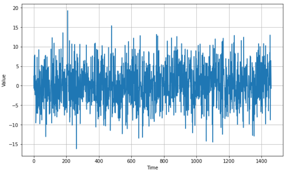
d. White Noise

# white noise
def white_noise(time, noise_level=1, seed=None):
    rnd = np.random.RandomState(seed)
    return rnd.randn(len(time)) * noise_level

noise_level = 5
noise = white_noise(time, noise_level, seed=42)
plot_series(time, noise)

e. Autocorrelation

# autocorrelation
def autocorrelation(time, amplitude, seed=None):
    rnd = np.random.RandomState(seed)
    φ1 = 0.5
    φ2 = -0.1
    ar = rnd.randn(len(time) + 50)
    ar[:50] = 100
    for step in range(50, len(time) + 50):
        ar[step] += φ1 * ar[step - 50]
        ar[step] += φ2 * ar[step - 33]
    return ar[50:] * amplitude

def autocorrelation(time, amplitude, seed=None):
    rnd = np.random.RandomState(seed)
    φ = 0.8
    ar = rnd.randn(len(time) + 1)
    for step in range(1, len(time) + 1):
        ar[step] += φ * ar[step - 1]
    return ar[1:] * amplitude

series = autocorrelation(time, amplitude, seed=42)
plot_series(time[:200], series[:200])

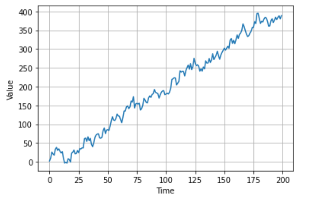
f. Autocorrelation and Trend

# autocorrelation + trend
series = autocorrelation(time, 10, seed=42) + trend(time, 2)
plot_series(time[:200], series[:200])

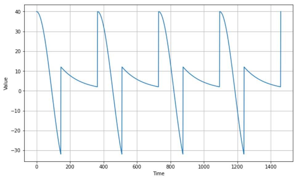
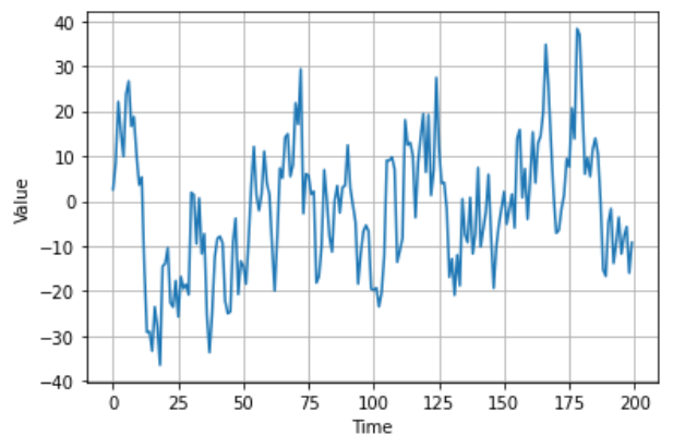
g. Autocorrelation and Seasonality

# autocorrelation + seasonality
series = autocorrelation(time, 10, seed=42) + seasonality(time, period=50, amplitude=150) + trend(time, 2)
plot_series(time[:200], series[:200])

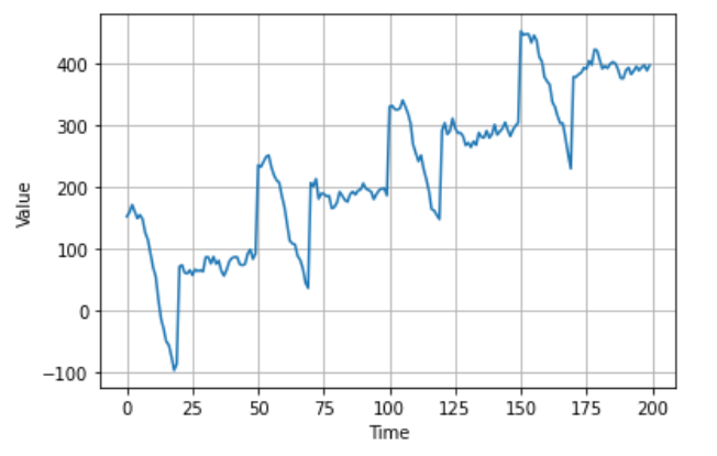
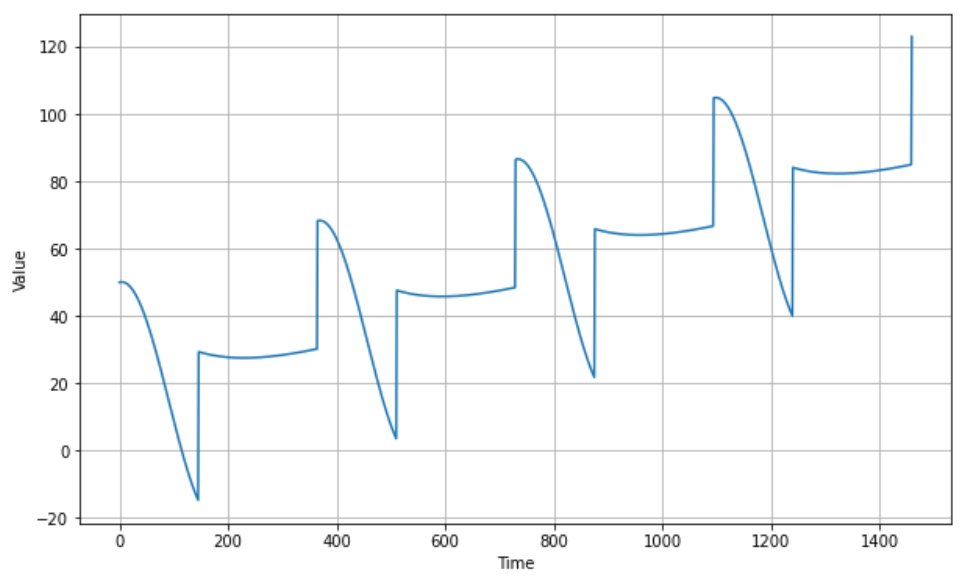
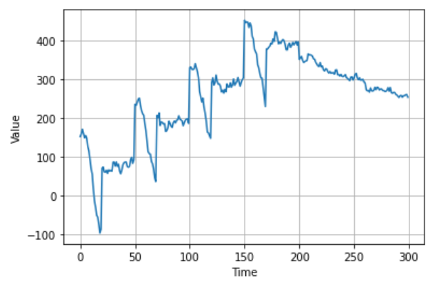
h. Autocorrelation and Autocorrelation

# autocorrelation + autocorrelation
series = autocorrelation(time, 10, seed=42) + seasonality(time, period=50, amplitude=150) + trend(time, 2)
series2 = autocorrelation(time, 5, seed=42) + seasonality(time, period=50, amplitude=2) + trend(time, -1) + 550
series[200:] = series2[200:]
#series += noise(time, 30)
plot_series(time[:300], series[:300])

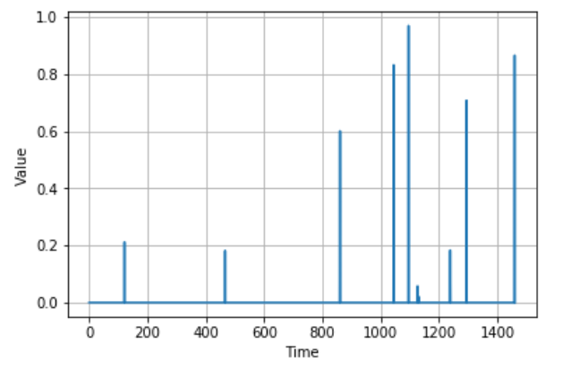
i. Impulses

# impulses
def impulses(time, num_impulses, amplitude=1, seed=None):
    rnd = np.random.RandomState(seed)
    impulse_indices = rnd.randint(len(time), size=10)
    series = np.zeros(len(time))
    for index in impulse_indices:
        series[index] += rnd.rand() * amplitude
    return series    

series = impulses(time, 10, seed=42)
plot_series(time, series)

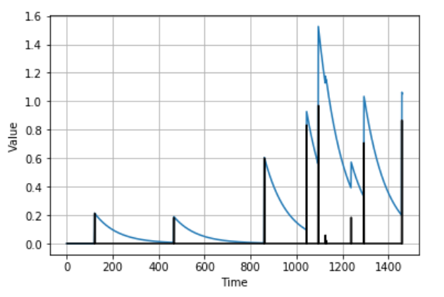
j. Autocorrelation and Impulses

# autocorrelation + impulses
def autocorrelation(source, φs):
    ar = source.copy()
    max_lag = len(φs)
    for step, value in enumerate(source):
        for lag, φ in φs.items():
            if step - lag > 0:
              ar[step] += φ * ar[step - lag]
    return ar

signal = impulses(time, 10, seed=42)
series = autocorrelation(signal, {1: 0.99})
plot_series(time, series)
plt.plot(time, signal, "k-")
plt.show()S

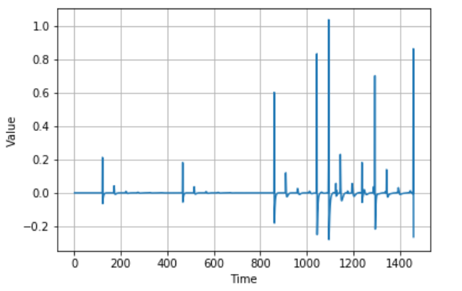
series_diff1 = series[1:] - series[:-1]
plot_series(time[1:], series_diff1)

2. DNN

# Data preparation
def window_dataset(series, window_size, batch_size, shuffle_buffer):
    dataset = tf.data.Dataset.from_tensor_slices(series)
    dataset = dataset.window(window_size + 1, shift=1, drop_remainder=True)
    dataset = dataset.flat_map(lambda window : window.batch(window_size + 1))
    dataset = dataset.shuffle(shuffle_buffer).map(lambda window : (window[:-1], window[-1]))
    dataset = dataset.batch(batch_size).prefetch(1)
    return dataset

# Forecast
forecast = []

for time in range(len(series) - window_size):
    if time == 0:
        print(series[time:time + window_size][np.newaxis])
    forecast.append(model.predict(series[time:time + window_size][np.newaxis]))

forecast = forecast[split_time-window_size:]
print(forecast)
results = np.array(forecast)[:, 0, 0]

# Callbacks
model = tf.keras.models.Sequential([
    tf.keras.layers.Dense(10, input_shape=[window_size], activation='relu'),
    tf.keras.layers.Dense(10, activation='relu'),
    tf.keras.layers.Dense(1)
])

lr_schedule = tf.keras.callbacks.LearningRateScheduler(
    lambda epoch : 1e-8 * 10 ** (epoch / 20)
)
optimizer = tf.keras.optimizers.SGD(lr=1e-8, momentum=0.9)
model.compile(loss='mse', optimizer=optimizer)
history = model.fit(dataset, epochs=100, callbacks=[lr_schedule], verbose=0)

lrs = 1e-8 * 10 ** (np.arange(100) / 20)
plt.figure()
plt.semilogx(lrs, history.history['loss'])
plt.axis([1e-8, 1e-3, 0, 30])
plt.show()

3. RNN

# Simple RNN

tf.keras.backend.clear_session()
tf.random.set_seed(51)
np.random.seed(51)

model = tf.keras.models.Sequential([
    tf.keras.layers.Lambda(lambda x : tf.expand_dims(x, axis=-1), input_shape=[None]),
    tf.keras.layers.SimpleRNN(40, return_sequences=True),
    tf.keras.layers.SimpleRNN(40),
    tf.keras.layers.Dense(1),
    tf.keras.layers.Lambda(lambda x : x * 100.0)
])
optimizer = tf.keras.optimizers.SGD(lr=5e-5, momentum=0.9)
model.compile(loss=tf.keras.losses.Huber(),
              optimizer=optimizer,
              metrics=['mae'])
history = model.fit(dataset, epochs=400)

# LSTM
model = tf.keras.models.Sequential([
    tf.keras.layers.Lambda(lambda x : tf.expand_dims(x, axis=-1), input_shape=[None]),
    tf.keras.layers.Bidirectional(tf.keras.layers.LSTM(32, return_sequences=True)),
    tf.keras.layers.Bidirectional(tf.keras.layers.LSTM(32)),
    tf.keras.layers.Dense(1),
    tf.keras.layers.Lambda(lambda x : x * 100.0)
])

4. Sunspots

# data preparation
def windowed_dataset(series, window_size, batch_size, shuffle_buffer):
    series = tf.expand_dims(series, axis=-1)
    ds = tf.data.Dataset.from_tensor_slices(series)
    ds = ds.window(window_size + 1, shift=1, drop_remainder=True)
    ds = ds.flat_map(lambda w: w.batch(window_size + 1))
    ds = ds.shuffle(shuffle_buffer)
    ds = ds.map(lambda w: (w[:-1], w[1:]))
    return ds.batch(batch_size).prefetch(1)

# forecast function
def model_forecast(model, series, window_size):
    ds = tf.data.Dataset.from_tensor_slices(series)
    ds = ds.window(window_size, shift=1, drop_remainder=True)
    ds = ds.flat_map(lambda w: w.batch(window_size))
    ds = ds.batch(32).prefetch(1)
    forecast = model.predict(ds)
    return forecast

# model
tf.keras.backend.clear_session()
tf.random.set_seed(51)
np.random.seed(51)
train_set = windowed_dataset(x_train, window_size=60, batch_size=100, shuffle_buffer=shuffle_buffer_size)

model = tf.keras.models.Sequential([
  tf.keras.layers.Conv1D(filters=60, kernel_size=5,
                      strides=1, padding="causal",
                      activation="relu",
                      input_shape=[None, 1]),
  tf.keras.layers.LSTM(60, return_sequences=True),
  tf.keras.layers.LSTM(60, return_sequences=True),
  tf.keras.layers.Dense(30, activation="relu"),
  tf.keras.layers.Dense(10, activation="relu"),
  tf.keras.layers.Dense(1),
  tf.keras.layers.Lambda(lambda x: x * 400)
])

optimizer = tf.keras.optimizers.SGD(lr=1e-5, momentum=0.9)
model.compile(loss=tf.keras.losses.Huber(),
              optimizer=optimizer,
              metrics=["mae"])
history = model.fit(train_set,epochs=500)

# forecast
rnn_forecast = model_forecast(model, series[..., np.newaxis], window_size)
rnn_forecast = rnn_forecast[split_time - window_size:-1, -1, 0]