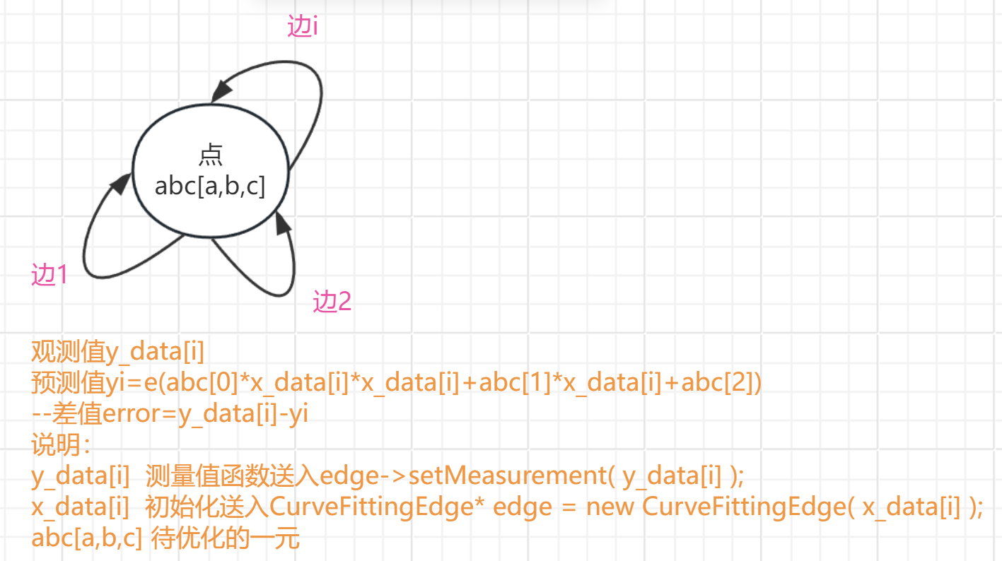
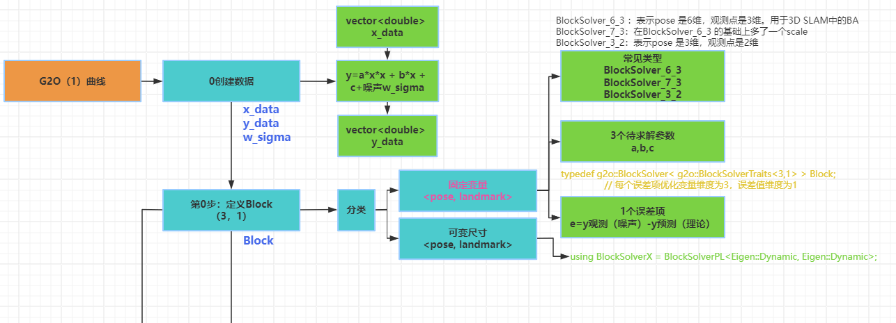
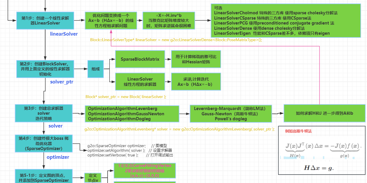
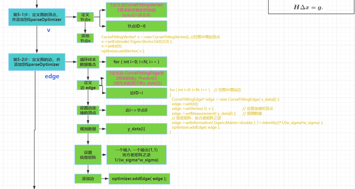
g2o（2）求解曲线y=exp(ax2+bx+c)

 

https://mp.weixin.qq.com/s?__biz=MzIxOTczOTM4NA==&mid=2247486858&idx=1&sn=ce458d5eb6b1ad11b065d71899e31a04&chksm=97d7e81da0a0610b1e3e12415b6de1501329920c3074ab5b48e759edbb33d264a73f1a9f9faf&scene=21#wechat_redirect

简要流程

0-0获取数据 x 和 y

0-1确定要优化的量a ,b, c

1-1 获取理论模型 y=ax^2+bx+c

1-2 确定误差方程e =min||f(x+Δx)-f(x)||

2 根据误差方程e确定一阶导J=2ax+b和二阶导H=2a 矩阵，信息矩阵  

3 根据误差方程e , 求解模型（例如高斯牛顿）确定 H和g表达形式

   构造 H *Δx= g最小二乘 

    J(x)*J(x)*Δx=-J(x) f(x)

        H* Δx = g

4 求解 Δx=H.inv*g  确定求解H逆的方法

5 跟新 x=x+Δx

6 求解 e =f(x+Δx)-f(x)误差

7 迭代直到小于阈值或者总次数

 

 

 

 

 

 

 

源码地址

G2O代码

CMakeLists.txt

?

1 2 3 4 5 6 7 8 9 10 11 12 13 14 15 16 17 18 19 20 21 22 23 24 25 26

cmake_minimum_required( VERSION 2.8 ) project( g2o_curve_fitting )   set( CMAKE_BUILD_TYPE "Release" ) set( CMAKE_CXX_FLAGS "-std=c++11 -O3" )   # 添加cmake模块以使用ceres库 list( APPEND CMAKE_MODULE_PATH ${PROJECT_SOURCE_DIR}/cmake_modules )   # 寻找G2O find_package( G2O REQUIRED ) include_directories(     ${G2O_INCLUDE_DIRS}     "/usr/include/eigen3" )   # OpenCV find_package( OpenCV REQUIRED ) include_directories( ${OpenCV_DIRS} )   add_executable( curve_fitting main.cpp ) # 与G2O和OpenCV链接 target_link_libraries( curve_fitting     ${OpenCV_LIBS}     g2o_core g2o_stuff )

　　

main.cpp

?

1 2 3 4 5 6 7 8 9 10 11 12 13 14 15 16 17 18 19 20 21 22 23 24 25 26 27 28 29 30 31 32 33 34 35 36 37 38 39 40 41 42 43 44 45 46 47 48 49 50 51 52 53 54 55 56 57 58 59 60 61 62 63 64 65 66 67 68 69 70 71 72 73 74 75 76 77 78 79 80 81 82 83 84 85 86 87 88 89 90 91 92 93 94 95 96 97 98 99 100 101 102 103 104 105 106 107 108 109 110 111 112 113 114 115 116 117

#include <iostream> #include <g2o/core/base_vertex.h> #include <g2o/core/base_unary_edge.h> #include <g2o/core/block_solver.h> #include <g2o/core/optimization_algorithm_levenberg.h> #include <g2o/core/optimization_algorithm_gauss_newton.h> #include <g2o/core/optimization_algorithm_dogleg.h> #include <g2o/solvers/dense/linear_solver_dense.h> #include <Eigen/Core> #include <opencv2/core/core.hpp> #include <cmath> #include <chrono> using namespace std;   // 曲线模型的顶点，模板参数：优化变量维度和数据类型 class CurveFittingVertex: public g2o::BaseVertex<3, Eigen::Vector3d> { public:     EIGEN_MAKE_ALIGNED_OPERATOR_NEW     virtual void setToOriginImpl() // 重置     {         _estimate << 0,0,0;     }           virtual void oplusImpl( const double* update ) // 更新     {<br>         _estimate += Eigen::Vector3d(update);     }     // 存盘和读盘：留空     virtual bool read( istream& in ) {}     virtual bool write( ostream& out ) const {} };   // 误差模型 模板参数：观测值维度，类型，连接顶点类型 class CurveFittingEdge: public g2o::BaseUnaryEdge<1,double,CurveFittingVertex> { public:     EIGEN_MAKE_ALIGNED_OPERATOR_NEW     CurveFittingEdge( double x ): BaseUnaryEdge(), _x(x) {}     // 计算曲线模型误差     void computeError()     {         const CurveFittingVertex* v = static_cast<const CurveFittingVertex*> (_vertices[0]);         const Eigen::Vector3d abc = v->estimate();         _error(0,0) = _measurement - std::exp( abc(0,0)*_x*_x + abc(1,0)*_x + abc(2,0) ) ;     }     virtual bool read( istream& in ) {}     virtual bool write( ostream& out ) const {} public:     double _x;  // x 值， y 值为 _measurement };   int main( int argc, char** argv ) {     double a=1.0, b=2.0, c=1.0;         // 真实参数值     int N=100;                          // 数据点     double w_sigma=1.0;                 // 噪声Sigma值     cv::RNG rng;                        // OpenCV随机数产生器     double abc[3] = {0,0,0};            // abc参数的估计值       vector<double> x_data, y_data;      // 数据           cout<<"generating data: "<<endl;     for ( int i=0; i<N; i++ )     {         double x = i/100.0;         x_data.push_back ( x );         y_data.push_back (             exp ( a*x*x + b*x + c ) + rng.gaussian ( w_sigma )         );         cout<<x_data[i]<<" "<<y_data[i]<<endl;     }           // 构建图优化，先设定g2o     typedef g2o::BlockSolver< g2o::BlockSolverTraits<3,1> > Block;  // 每个误差项优化变量维度为3，误差值维度为1     Block::LinearSolverType* linearSolver = new g2o::LinearSolverDense<Block::PoseMatrixType>(); // 线性方程求解器     Block* solver_ptr = new Block( linearSolver );      // 矩阵块求解器     // 梯度下降方法，从GN, LM, DogLeg 中选     g2o::OptimizationAlgorithmLevenberg* solver = new g2o::OptimizationAlgorithmLevenberg( solver_ptr );     // g2o::OptimizationAlgorithmGaussNewton* solver = new g2o::OptimizationAlgorithmGaussNewton( solver_ptr );     // g2o::OptimizationAlgorithmDogleg* solver = new g2o::OptimizationAlgorithmDogleg( solver_ptr );     g2o::SparseOptimizer optimizer;     // 图模型     optimizer.setAlgorithm( solver );   // 设置求解器     optimizer.setVerbose( true );       // 打开调试输出           // 往图中增加顶点     CurveFittingVertex* v = new CurveFittingVertex();     v->setEstimate( Eigen::Vector3d(0,0,0) );     v->setId(0);     optimizer.addVertex( v );           // 往图中增加边     for ( int i=0; i<N; i++ )     {         CurveFittingEdge* edge = new CurveFittingEdge( x_data[i] );         edge->setId(i);         edge->setVertex( 0, v );                // 设置连接的顶点         edge->setMeasurement( y_data[i] );      // 观测数值         edge->setInformation( Eigen::Matrix<double,1,1>::Identity()*1/(w_sigma*w_sigma) ); // 信息矩阵：协方差矩阵之逆         optimizer.addEdge( edge );     }           // 执行优化     cout<<"start optimization"<<endl;     chrono::steady_clock::time_point t1 = chrono::steady_clock::now();     optimizer.initializeOptimization();     optimizer.optimize(100);     chrono::steady_clock::time_point t2 = chrono::steady_clock::now();     chrono::duration<double> time_used = chrono::duration_cast<chrono::duration<double>>( t2-t1 );     cout<<"solve time cost = "<<time_used.count()<<" seconds. "<<endl;           // 输出优化值     Eigen::Vector3d abc_estimate = v->estimate();     cout<<"estimated model: "<<abc_estimate.transpose()<<endl;           return 0; }

　　

ceres代码

CMakeLists.txt

?

1 2 3 4 5 6 7 8 9 10 11 12 13 14 15 16 17 18 19 20

cmake_minimum_required( VERSION 2.8 ) project( ceres_curve_fitting )   set( CMAKE_BUILD_TYPE "Release" ) set( CMAKE_CXX_FLAGS "-std=c++11 -O3" )   # 添加cmake模块以使用ceres库 list( APPEND CMAKE_MODULE_PATH ${PROJECT_SOURCE_DIR}/cmake_modules )   # 寻找Ceres库并添加它的头文件 find_package( Ceres REQUIRED ) include_directories( ${CERES_INCLUDE_DIRS} )   # OpenCV find_package( OpenCV REQUIRED ) include_directories( ${OpenCV_DIRS} )   add_executable( curve_fitting main.cpp ) # 与Ceres和OpenCV链接 target_link_libraries( curve_fitting ${CERES_LIBRARIES} ${OpenCV_LIBS} )

　　

main.cpp

?

1 2 3 4 5 6 7 8 9 10 11 12 13 14 15 16 17 18 19 20 21 22 23 24 25 26 27 28 29 30 31 32 33 34 35 36 37 38 39 40 41 42 43 44 45 46 47 48 49 50 51 52 53 54 55 56 57 58 59 60 61 62 63 64 65 66 67 68 69 70 71 72 73 74 75 76 77 78

#include <iostream> #include <opencv2/core/core.hpp> #include <ceres/ceres.h> #include <chrono>   using namespace std;   // 代价函数的计算模型 struct CURVE_FITTING_COST {     CURVE_FITTING_COST ( double x, double y ) : _x ( x ), _y ( y ) {}     // 残差的计算     template <typename T>     bool operator() (         const T* const abc,     // 模型参数，有3维         T* residual ) const     // 残差     {         residual[0] = T ( _y ) - ceres::exp ( abc[0]*T ( _x ) *T ( _x ) + abc[1]*T ( _x ) + abc[2] ); // y-exp(ax^2+bx+c)         return true;     }     const double _x, _y;    // x,y数据 };   int main ( int argc, char** argv ) {     double a=1.0, b=2.0, c=1.0;         // 真实参数值     int N=100;                          // 数据点     double w_sigma=1.0;                 // 噪声Sigma值     cv::RNG rng;                        // OpenCV随机数产生器     double abc[3] = {0,0,0};            // abc参数的估计值       vector<double> x_data, y_data;      // 数据       cout<<"generating data: "<<endl;     for ( int i=0; i<N; i++ )     {         double x = i/100.0;         x_data.push_back ( x );         y_data.push_back (             exp ( a*x*x + b*x + c ) + rng.gaussian ( w_sigma )         );         cout<<x_data[i]<<" "<<y_data[i]<<endl;     }       // 构建最小二乘问题     ceres::Problem problem;     for ( int i=0; i<N; i++ )     {         problem.AddResidualBlock (     // 向问题中添加误差项         // 使用自动求导，模板参数：误差类型，输出维度，输入维度，维数要与前面struct中一致             new ceres::AutoDiffCostFunction<CURVE_FITTING_COST, 1, 3> (                 new CURVE_FITTING_COST ( x_data[i], y_data[i] )             ),             nullptr,            // 核函数，这里不使用，为空             abc                 // 待估计参数         );     }       // 配置求解器     ceres::Solver::Options options;     // 这里有很多配置项可以填     options.linear_solver_type = ceres::DENSE_QR;  // 增量方程如何求解     options.minimizer_progress_to_stdout = true;   // 输出到cout       ceres::Solver::Summary summary;                // 优化信息     chrono::steady_clock::time_point t1 = chrono::steady_clock::now();     ceres::Solve ( options, &problem, &summary );  // 开始优化     chrono::steady_clock::time_point t2 = chrono::steady_clock::now();     chrono::duration<double> time_used = chrono::duration_cast<chrono::duration<double>>( t2-t1 );     cout<<"solve time cost = "<<time_used.count()<<" seconds. "<<endl;       // 输出结果     cout<<summary.BriefReport() <<endl;     cout<<"estimated a,b,c = ";     for ( auto a:abc ) cout<<a<<" ";     cout<<endl;       return 0; }

　　

 

 

手撕代码

https://liuxiaofei.com.cn/blog/g2o%E4%BC%98%E5%8C%96%E8%A7%A3%E6%9E%90-%E6%89%8B%E5%8A%A8%E5%BE%AE%E5%88%86/

 

代码

?

1 2 3 4 5 6 7 8 9 10 11 12 13 14 15 16 17 18 19 20 21 22 23 24 25 26 27 28 29 30 31 32 33 34 35 36 37 38 39 40 41 42 43 44 45 46 47 48 49 50 51 52 53 54 55 56 57 58 59 60 61 62 63 64 65 66 67 68 69 70 71 72 73 74 75 76 77 78 79 80 81 82 83 84 85 86 87 88 89 90 91 92 93 94 95 96 97 98 99 100 101 102 103 104 105 106 107 108 109 110 111 112 113 114 115 116 117 118 119 120 121 122 123 124 125 126 127 128 129

#include <iostream> #include <g2o/core/g2o_core_api.h> #include <g2o/core/base_vertex.h> #include <g2o/core/base_unary_edge.h> #include <g2o/core/block_solver.h> #include <g2o/core/optimization_algorithm_levenberg.h> #include <g2o/core/optimization_algorithm_gauss_newton.h> #include <g2o/core/optimization_algorithm_dogleg.h> #include <g2o/solvers/dense/linear_solver_dense.h> #include <g2o/stuff/sampler.h> #include <Eigen/Core> #include <cmath> #include <chrono>    using namespace std;    // 曲线模型的顶点，模板参数：优化变量维度和数据类型 class CurveFittingVertex : public g2o::BaseVertex<3, Eigen::Vector3d> { public:   EIGEN_MAKE_ALIGNED_OPERATOR_NEW      // 重置   virtual void setToOriginImpl() override {     _estimate << 0, 0, 0;   }      // 更新，每一轮迭代后更新参数的值Δx。   virtual void oplusImpl(const double *update) override {     _estimate += Eigen::Vector3d(update);   }      // 存盘和读盘：留空   virtual bool read(istream &in) {}      virtual bool write(ostream &out) const {} };    // 误差模型 模板参数：观测值维度，类型，连接顶点类型 class CurveFittingEdge : public g2o::BaseUnaryEdge<1, double, CurveFittingVertex> { public:   EIGEN_MAKE_ALIGNED_OPERATOR_NEW      CurveFittingEdge(double x) : BaseUnaryEdge(), _x(x) {}      // 计算曲线模型误差，测量值减去估计值得到误差。   virtual void computeError() override {     const CurveFittingVertex *v = static_cast<const CurveFittingVertex *> (_vertices[0]);     const Eigen::Vector3d abc = v->estimate();     _error(0, 0) = _measurement - std::exp(abc(0, 0) * _x * _x + abc(1, 0) * _x + abc(2, 0));   }      // 计算雅可比矩阵，和上一篇高斯牛顿法里面的求解方式是一样的。   virtual void linearizeOplus() override {     const CurveFittingVertex *v = static_cast<const CurveFittingVertex *> (_vertices[0]);     const Eigen::Vector3d abc = v->estimate();     double y = exp(abc[0] * _x * _x + abc[1] * _x + abc[2]);     _jacobianOplusXi[0] = -_x * _x * y;     _jacobianOplusXi[1] = -_x * y;     _jacobianOplusXi[2] = -y;   }      virtual bool read(istream &in) {}      virtual bool write(ostream &out) const {}    public:   double _x;  // x 值， y 值为 _measurement };    int main(int argc, char **argv) {   double ar = 1.0, br = 2.0, cr = 1.0;         // 真实参数值   double ae = 2.0, be = -1.0, ce = 5.0;        // 估计参数值   int N = 100;                                 // 数据点   double w_sigma = 1.0;                        // 噪声Sigma值   double inv_sigma = 1.0 / w_sigma;   g2o::Sampler::seedRand();      vector<double> x_data, y_data;      // 数据   for (int i = 0; i < N; i++) {     double x = i / 100.0;     x_data.push_back(x);     y_data.push_back(exp(ar * x * x + br * x + cr) + g2o::Sampler::gaussRand(0, 0.02));//加上一个高斯误差，来表示测量是不准确的。   }      // 构建图优化，先设定g2o   typedef g2o::BlockSolver<g2o::BlockSolverTraits<3, 1>> BlockSolverType;  // 每个误差项优化变量维度为3，误差值维度为1   typedef g2o::LinearSolverDense<BlockSolverType::PoseMatrixType> LinearSolverType; // 线性求解器类型      // 梯度下降方法，可以从GN, LM, DogLeg 中选   auto solver = new g2o::OptimizationAlgorithmGaussNewton(     g2o::make_unique<BlockSolverType>(g2o::make_unique<LinearSolverType>()));   g2o::SparseOptimizer optimizer;     // 图模型   optimizer.setAlgorithm(solver);   // 设置求解器   optimizer.setVerbose(true);       // 打开调试输出      // 往图中增加顶点：待优化的参数。   //图优化的原理就是：不停的调整顶点位姿（参数）来使连接到顶点的边（误差函数）最优。   CurveFittingVertex *v = new CurveFittingVertex();   v->setEstimate(Eigen::Vector3d(ae, be, ce));   v->setId(0);   optimizer.addVertex(v);      // 往图中增加边：每个误差函数   for (int i = 0; i < N; i++) {     CurveFittingEdge *edge = new CurveFittingEdge(x_data[i]);     edge->setId(i);     edge->setVertex(0, v);                // 设置连接的顶点     edge->setMeasurement(y_data[i]);      // 观测数值 // 信息矩阵：协方差矩阵之逆，乘上一阶导数值用来决定当前梯度对全局梯度的贡献度。信息越清晰表明当前梯度越重要。 // 即人为的根据先验概率控制误差函数的权重。     edge->setInformation(Eigen::Matrix<double, 1, 1>::Identity() * 1 / (w_sigma * w_sigma));     optimizer.addEdge(edge);   }      // 执行优化   cout << "start optimization" << endl;   chrono::steady_clock::time_point t1 = chrono::steady_clock::now();   optimizer.initializeOptimization();   optimizer.optimize(10);   chrono::steady_clock::time_point t2 = chrono::steady_clock::now();   chrono::duration<double> time_used = chrono::duration_cast<chrono::duration<double>>(t2 - t1);   cout << "solve time cost = " << time_used.count() << " seconds. " << endl;      // 输出优化值   Eigen::Vector3d abc_estimate = v->estimate();   cout << "estimated model: " << abc_estimate.transpose() << endl;      return 0; }