对比学习简记

目录

• Self-Supervised Learning 的核心思想
  • 两大主流方法
  • 实践应用
• Contrastive Representation Learning
  • 对比学习目标函数
    • Contrastive Loss
    • Triplet Loss
    • N-pair Loss
    • NCE
    • InfoNCE
  • 对比学习关键点
    • 数据增强
    • 大的BatchSize
    • hard Negative Mining
  • vision
    • Image Augmentation
    • SimCLR
    • CLIP
  • nlp
    • Text Augmentation
    • SimCSE
  • References

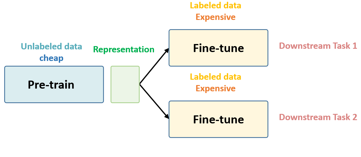
Self-Supervised Learning 的核心思想

Unsupervised Pre-train, Supervised Fine-tune.

两大主流方法

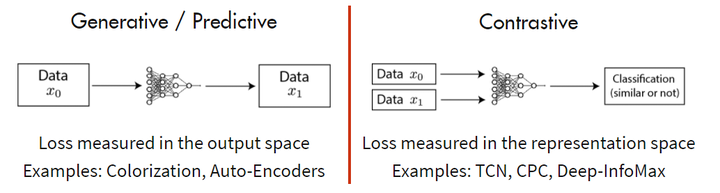
• 基于 Generative 的方法
• 基于 Contrative 的方法

基于 Generative 的方法主要关注的重建误差，还原原始输入；

基于Contrastive 的方法不要求模型能够重建原始输入，而是希望模型能够在特征空间上对不同的输入进行分辨，判断输入是否相似。

实践应用

• BERT系列：nlp
• VIT系列：cv
• data2vec系列：multimodal
• SimCLR系列：对比学习
• MoCo系列

Contrastive Representation Learning

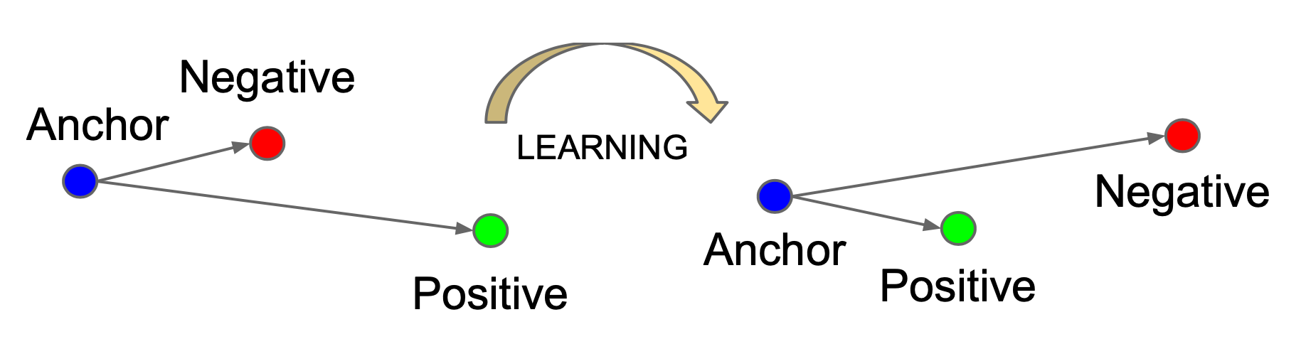
对比学习指导原则

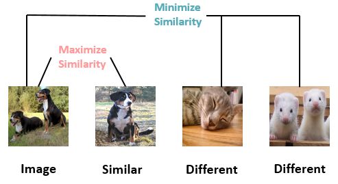
• 构造相似实例和不相似实例
• 习得一个表示学习模型，使得相似的实例在投影空间中比较接近，而不相似的实例在投影空间中距离比较远

对比学习目标函数

Contrastive Loss

最早的Loss是对比Loss，即同类样本间更相似，最小化同类样本的embedding 距离，最大化非同类embedding的距离

\[\mathcal{L}_\text{cont}(\mathbf{x}_i, \mathbf{x}_j, \theta) = \mathbb{1}[y_i=y_j] \| f_\theta(\mathbf{x}_i) - f_\theta(\mathbf{x}_j) \|^2_2 + \mathbb{1}[y_i\neq y_j]\max(0, \epsilon - \|f_\theta(\mathbf{x}_i) - f_\theta(\mathbf{x}_j)\|_2)^2 \]

Triplet Loss

Triplet loss最小化anchor和正样本间的距离，最大化anchor和负样本间的距离

\[\mathcal{L}_\text{triplet}(\mathbf{x}, \mathbf{x}^+, \mathbf{x}^-) = \sum_{\mathbf{x} \in \mathcal{X}} \max\big( 0, \|f(\mathbf{x}) - f(\mathbf{x}^+)\|^2_2 - \|f(\mathbf{x}) - f(\mathbf{x}^-)\|^2_2 + \epsilon \big) \]

关键：选择合适的负样本，提升模型性能

N-pair Loss

Multi-Class N-pair loss generalizes triplet loss to include comparison with multiple negative samples.

Given a \((N + 1)\) tuplet of training samples,\(\{ \mathbf{x}, \mathbf{x}^+, \mathbf{x}^-_1, \dots, \mathbf{x}^-_{N-1} \}\), including one positive and \(N-1\) negative ones, N-pair loss is defined as:

\[\begin{aligned} \mathcal{L}_\text{N-pair}(\mathbf{x}, \mathbf{x}^+, \{\mathbf{x}^-_i\}^{N-1}_{i=1}) &= \log\big(1 + \sum_{i=1}^{N-1} \exp(f(\mathbf{x})^\top f(\mathbf{x}^-_i) - f(\mathbf{x})^\top f(\mathbf{x}^+))\big) \\ &= -\log\frac{\exp(f(\mathbf{x})^\top f(\mathbf{x}^+))}{\exp(f(\mathbf{x})^\top f(\mathbf{x}^+)) + \sum_{i=1}^{N-1} \exp(f(\mathbf{x})^\top f(\mathbf{x}^-_i))} \end{aligned} \]

当负样本数量为1时，等价于多分类softmax。

NCE

把多分类问题转化成二分类，判断正样本和负样本是否为同一类。

\[\begin{aligned} \mathcal{L}_\text{NCE} &= - \frac{1}{N} \sum_{i=1}^N \big[ \log \sigma (\ell_\theta(\mathbf{x}_i)) + \log (1 - \sigma (\ell_\theta(\tilde{\mathbf{x}}_i))) \big] \\ \text{ where }\sigma(\ell) &= \frac{1}{1 + \exp(-\ell)} = \frac{p_\theta}{p_\theta + q} \end{aligned} \]

其中 target sample \(\sim P(\mathbf{x} \vert C=1; \theta) = p_\theta(\mathbf{x})\), noise sample \(\sim P(\tilde{\mathbf{x}} \vert C=0) = q(\tilde{\mathbf{x}})\).

InfoNCE

\[\mathcal{L}_q = - \log\dfrac{\exp(q k_+ / \tau)}{\sum_i \exp(q k_i / \tau)} \]

假设我们忽略\(\tau\)，那么infoNCE loss其实就是cross entropy loss。唯一的区别是，在cross entropy loss里，\(k\)

指代的是数据集里类别的数量，而在对比学习InfoNCE loss里，这个\(k\)指的是负样本的数量.

如果温度系数设的越大，logits分布变得越平滑，那么对比损失会对所有的负样本一视同仁，导致模型学习没有轻重。如果温度系数设的过小，则模型会越关注特别困难的负样本，但其实那些负样本很可能是潜在的正样本，这样会导致模型很难收敛或者泛化能力差.

对比学习损失（InfoNCE loss）与交叉熵损失的联系，以及温度系数的作用 - Youngshell的文章 - 知乎 https://zhuanlan.zhihu.com/p/506544456

对比学习关键点

数据增强

对原始数据增加噪音等数据增强，生成正样本。

如SimCLR表明，随机裁剪和随机颜色失真对视觉表示学习非常关键。

大的BatchSize

对依赖In-batchNegative的场景，大的batch size可以提高训练效率，增加模型挑战。

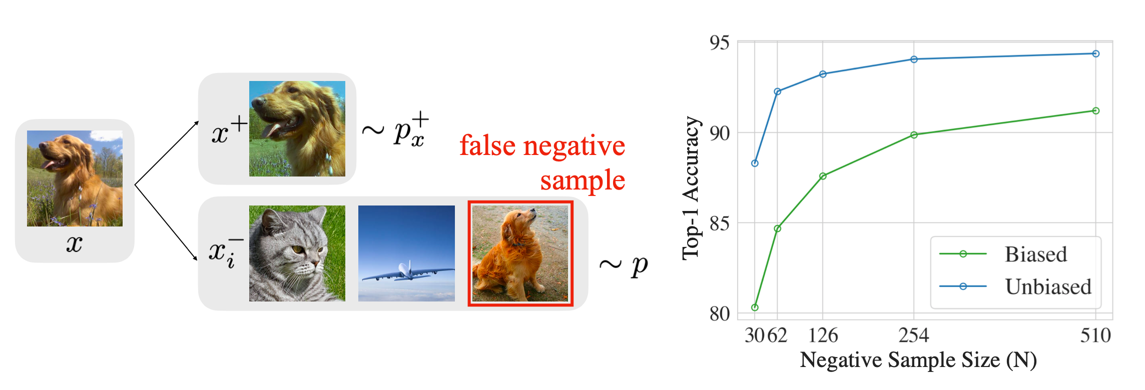
hard Negative Mining

对于有监督情况，可以直接将其它类样本作为负样本；

对于无监督情况，可能会偶然把同类样本作为负样本，导致性能大幅下降。

vision

Image Augmentation

裁剪、缩放、加噪、翻转、转换灰度图

常用框架：AutoAugment、RandAugment、PBA、UDA

图像混合

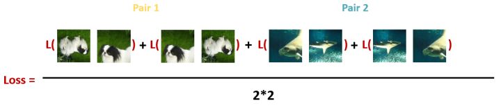
SimCLR

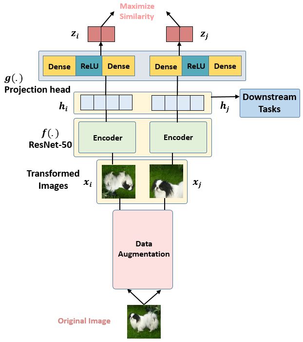
loss, 每个Batch里面的所有Pair的损失之和取平均:

\[L = \frac{1}{2N}\sum_{k=1}^{N}[l(2k-1,2k)+l(2k,2k-1)] \]

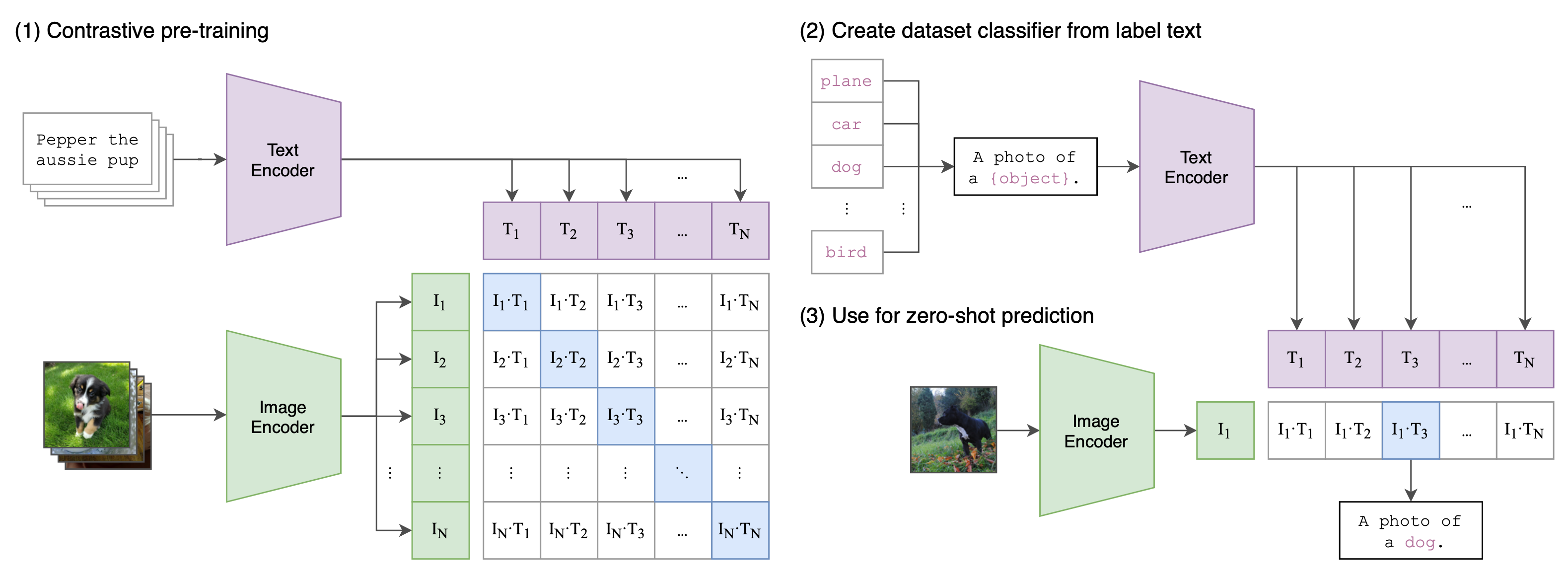
CLIP

nlp

Text Augmentation

编辑距离、随机替换、删除等

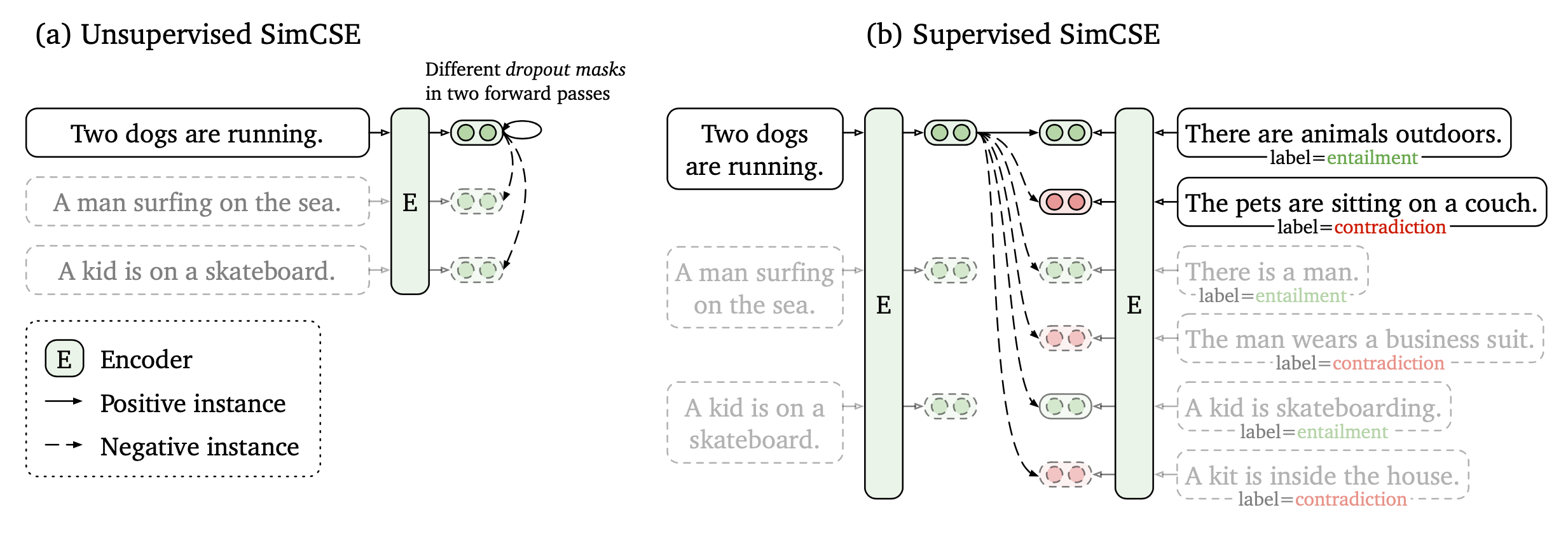
SimCSE

Unsupervised SimCSE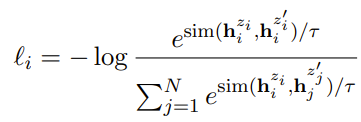

Supervised SimCSE

SimCSE2 中改进了两点：

1. 负样本质量，原本都是同一句话的embedding dropout，但句子长度相同，会导致模型倾向。
2. batchsize过大，引起性能下降，未解之谜

def unsup_loss(y_pred, lamda=0.05, device="cpu"):
    idxs = torch.arange(0, y_pred.shape[0], device=device)
    y_true = idxs + 1 - idxs % 2 * 2
    similarities = F.cosine_similarity(y_pred.unsqueeze(1), y_pred.unsqueeze(0), dim=2)

    similarities = similarities - torch.eye(y_pred.shape[0], device=device) * 1e12

    similarities = similarities / lamda

    loss = F.cross_entropy(similarities, y_true)
    return torch.mean(loss)


def sup_loss(y_pred, lamda=0.05, device="cpu"):
    row = torch.arange(0, y_pred.shape[0], 3, device=device)
    col = torch.arange(y_pred.shape[0], device=device)
    col = torch.where(col % 3 != 0)[0]
    y_true = torch.arange(0, len(col), 2, device=device)
    similarities = F.cosine_similarity(y_pred.unsqueeze(1), y_pred.unsqueeze(0), dim=2)

    similarities = torch.index_select(similarities, 0, row)
    similarities = torch.index_select(similarities, 1, col)

    similarities = similarities / lamda

    loss = F.cross_entropy(similarities, y_true)
    return torch.mean(loss)

References

【1】对比学习（Contrastive Learning）:研究进展精要. https://zhuanlan.zhihu.com/p/367290573

【2】https://lilianweng.github.io/posts/2021-05-31-contrastive/

【3】Self-Supervised Learning 超详细解读 (目录) - 科技猛兽的文章 - 知乎 https://zhuanlan.zhihu.com/p/381354026

【4】对比学习损失（InfoNCE loss）与交叉熵损失的联系，以及温度系数的作用 - Youngshell的文章 - 知乎 https://zhuanlan.zhihu.com/p/506544456