yolov5 筛选正样本流程 代码多图详解

yolov5正样本筛选原理
正样本全称是anchor正样本,正样本所指的对象是anchor box,即先验框。
先验框:从YOLO v2开始吸收了Faster RCNN的优点,设置了一定数量的预选框,使得模型不需要直接预测物体尺度与坐标,只需要预测先验框到真实物体的偏移,降低了预测难度。
正样本获取规则
Yolov5算法使用如下3种方式增加正样本个数:
一、跨anchor预测
假设一个GT框落在了某个预测分支的某个网格内,该网格具有3种不同大小anchor,若GT可以和这3种anchor中的多种anchor匹配,则这些匹配的anchor都可以来预测该GT框,即一个GT框可以使用多种anchor来预测。
具体方法:
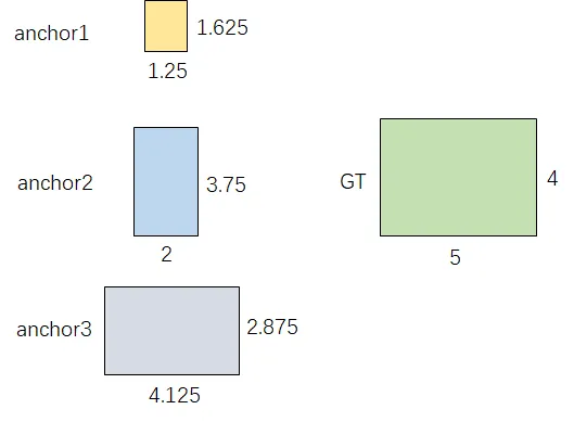
不同于IOU匹配,yolov5采用基于宽高比例的匹配策略,GT的宽高与anchors的宽高对应相除得到ratio1,anchors的宽高与GT的宽高对应相除得到ratio2,取ratio1和ratio2的最大值作为最后的宽高比,该宽高比和设定阈值(默认为4)比较,小于设定阈值的anchor则为匹配到的anchor。
anchor_boxes=torch.tensor([[1.25000, 1.62500],[2.00000, 3.75000],[4.12500, 2.87500]])
gt_box=torch.tensor([5,4])

ratio1=gt_box/anchor_boxes
ratio2=anchor_boxes/gt_box
ratio=torch.max(ratio1, ratio2).max(1)[0]
print(ratio)

anchor_t=4
res=ratio<anchor_t
print(res)
tensor([4.0000, 2.5000, 1.3913])
tensor([False,  True,  True])
与 GT 相匹配的的 anchor 为 **anchor2 **和 anchor3。
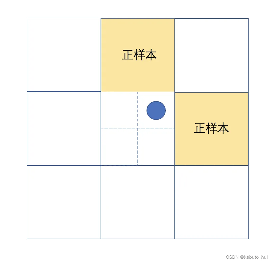
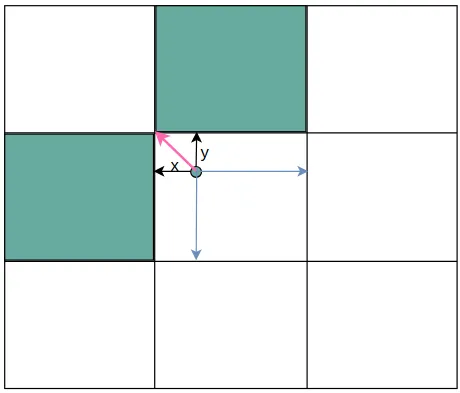
二、跨grid预测
假设一个GT框落在了某个预测分支的某个网格内,则该网格有左、上、右、下4个邻域网格,根据GT框的中心位置,将最近的2个邻域网格也作为预测网格,也即一个GT框可以由3个网格来预测。
计算例子:
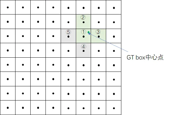
GT box中心点处于grid1中,grid1被选中。为了增加增样本,grid1的上下左右grid为候选网格,因为GT中心点更靠近grid2和grid3,grid2和grid3也作为匹配到的网格。
根据上个步骤中的anchor匹配结果,GT与anchor2、anchor3相匹配,因此GT在当前层匹配到的正样本有6个,分别为:
- grid1_anchor2,grid1_anchor3
- grid2_anchor2,grid2_anchor3
- grid3_anchor2,grid3_anchor3
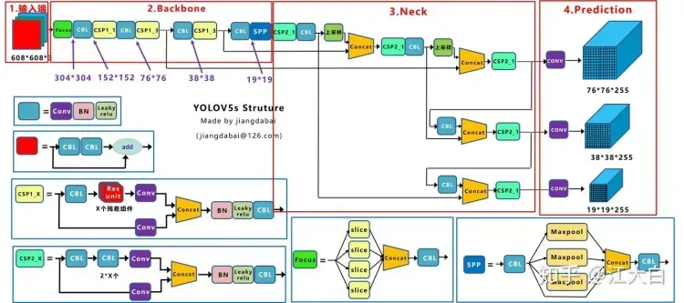
三、跨分支预测
假设一个GT框可以和2个甚至3个预测分支上的anchor匹配,则这2个或3个预测分支都可以预测该GT框。即一个GT框可以在3个预测分支上匹配正样本,在每一个分支上重复anchor匹配和grid匹配的步骤,最终可以得到某个GT 匹配到的所有正样本。
如下图在Prediction的3个不同尺度的输出中,gt都可以去匹配正样本。
正样本筛选
正样本筛选主要做了四件事情:
- 通过宽高比获得合适的anchor
- 通过anchor所在的网格获得上下左右扩展网格
- 获取标注框相对网格左上角的偏移量
- 返回获得的anchor,网格序号,偏移量,类别等
yolov5中anchor值
anchors:
  - [10,13, 16,30, 33,23]  # P3/8
  - [30,61, 62,45, 59,119]  # P4/16
  - [116,90, 156,198, 373,326]  # P5/32
yolov5的网络有三个尺寸的输出,不同大小的输出对应不同尺寸:
- 8倍下采样: [10,13, 16,30, 33,23]
- 16倍下采样:[30,61, 62,45, 59,119]
- 32倍下采样:[116,90, 156,198, 373,326]
注释代码
yolov5/utils/loss.py
    def build_targets(self, p, targets):
        # Build targets for compute_loss(), input targets(image,class,x,y,w,h)

        """
        p: 预测值
        targets:gt
        (Pdb) pp p[0].shape
        torch.Size([1, 3, 80, 80, 7])
        (Pdb) pp p[1].shape
        torch.Size([1, 3, 40, 40, 7])
        (Pdb) pp p[2].shape
        torch.Size([1, 3, 20, 20, 7])
        (Pdb) pp targets.shape
        torch.Size([23, 6])
        """
        na, nt = self.na, targets.shape[0]  # number of anchors, targets
        tcls, tbox, indices, anch = [], [], [], []

        """
        tcls    保存类别id
        tbox    保存的是gt中心相对于所在grid cell左上角偏移量。也会计算出gt中心相对扩展anchor的偏移量
        indices 保存的内容是:image_id, anchor_id, grid x刻度  grid y刻度
        anch 保存anchor的具体宽高
        """

        gain = torch.ones(7, device=self.device)  # normalized to gridspace gain
        ai = torch.arange(na, device=self.device).float().view(na, 1).repeat(1, nt)  # same as .repeat_interleave(nt)
        """
        (Pdb) ai
        tensor([[0., 0., 0., 0., 0., 0., 0., 0., 0., 0., 0., 0., 0., 0., 0., 0., 0., 0., 0., 0., 0., 0., 0.],
                [1., 1., 1., 1., 1., 1., 1., 1., 1., 1., 1., 1., 1., 1., 1., 1., 1., 1., 1., 1., 1., 1., 1.],
                [2., 2., 2., 2., 2., 2., 2., 2., 2., 2., 2., 2., 2., 2., 2., 2., 2., 2., 2., 2., 2., 2., 2.]], device='cuda:0')
        (Pdb) ai.shape
        torch.Size([3, 23])
        """
        targets = torch.cat((targets.repeat(na, 1, 1), ai[..., None]), 2)  # append anchor indices

        g = 0.5  # bias
        off = torch.tensor(
            [
                [0, 0],
                [1, 0],
                [0, 1],
                [-1, 0],
                [0, -1],  # j,k,l,m
                # [1, 1], [1, -1], [-1, 1], [-1, -1],  # jk,jm,lk,lm
            ],
            device=self.device).float() * g  # offsets

        for i in range(self.nl):
            anchors, shape = self.anchors[i], p[i].shape
            """
            (Pdb) anchors
            tensor([[1.25000, 1.62500],
                    [2.00000, 3.75000],
                    [4.12500, 2.87500]], device='cuda:0')
            (Pdb) shape
            torch.Size([1, 3, 80, 80, 7])
            """
            gain[2:6] = torch.tensor(shape)[[3, 2, 3, 2]]  # xyxy gain
            """
            (Pdb) gain
            tensor([ 1.,  1., 80., 80., 80., 80.,  1.], device='cuda:0')
            """

            # Match targets to anchors
            t = targets * gain  # shape(3,n,7)  # 将grid cell还原到当前feature map上
            """
            (Pdb) t.shape
            torch.Size([3, 23, 7])
            """

            if nt:
                # Matches
                r = t[..., 4:6] / anchors[:, None]  # wh ratio
                j = torch.max(r, 1 / r).max(2)[0] < self.hyp['anchor_t']  # compare
                # j = wh_iou(anchors, t[:, 4:6]) > model.hyp['iou_t']  # iou(3,n)=wh_iou(anchors(3,2), gwh(n,2))
                t = t[j]  # filter
                """
                (Pdb) t.shape
                torch.Size([3, 23, 7]) -> torch.Size([62, 7])
                """

                # Offsets
                gxy = t[:, 2:4]  # grid xy
                gxi = gain[[2, 3]] - gxy  # inverse
                j, k = ((gxy % 1 < g) & (gxy > 1)).T
                """
                (Pdb) ((gxy % 1 < g) & (gxy > 1)).shape
                torch.Size([186, 2])
                (Pdb) ((gxy % 1 < g) & (gxy > 1)).T.shape
                torch.Size([2, 186])
                """
                l, m = ((gxi % 1 < g) & (gxi > 1)).T

                j = torch.stack((torch.ones_like(j), j, k, l, m))
                """
                torch.ones_like(j) 代表gt中心所在grid cell
                j, k, l, m 代表扩展的上下左右grid cell

                torch.Size([5, 51])
                """
                t = t.repeat((5, 1, 1))[j]
                """
                标签也重复5次,和上面的扩展gird cell一起筛选出所有的,符合条件的grid cell
                (Pdb) pp t.shape
                torch.Size([153, 7])
                (Pdb) t.repeat((5, 1, 1)).shape
                torch.Size([5, 153, 7])
                (Pdb) pp t.shape
                torch.Size([232, 7])
                """
                offsets = (torch.zeros_like(gxy)[None] + off[:, None])[j]

                """
                计算出所有grid cell的偏移量,作用在标签上之后就能得到最终的grid cell
                (Pdb) pp offsets.shape
                torch.Size([529, 2])
                """
            else:
                t = targets[0]
                offsets = 0


            # Define
            bc, gxy, gwh, a = t.chunk(4, 1)  # (image, class), grid xy, grid wh, anchors
            a, (b, c) = a.long().view(-1), bc.long().T  # anchors, image, class
            gij = (gxy - offsets).long()
            """
            用gt中心点的坐标减去偏移量,得到最终的grid cell的坐标。其中中心点也在。
            gxy 是在当前feature map下的gt中心点,如80*80下的 (55.09, 36.23),减去偏移量,再取整就能得到一个grid cell的坐标,如 (55,36)
            Pdb) pp gij.shape
            torch.Size([529, 2])
            (Pdb) pp gij
            tensor([[ 9, 22],
                [ 2, 23],
                [ 6, 23],
                ...,
                [ 5, 19],
                [ 5, 38],
                [15, 36]], device='cuda:0')
            """
            gi, gj = gij.T  # grid indices

            # Append
            # indices 保存的内容是:image_id, anchor_id(0,1,2), grid x刻度  grid y刻度。这里的刻度就是正样本
            indices.append((b, a, gj.clamp_(0, shape[2] - 1), gi.clamp_(0, shape[3] - 1)))  # image, anchor, grid

            # tbox保存的是gt中心相对于所在grid cell左上角偏移量。也会计算出gt中心相对扩展anchor的偏移量
            tbox.append(torch.cat((gxy - gij, gwh), 1))  # box
            """
            (Pdb) pp tbox[0].shape
                torch.Size([312, 4])
            (Pdb) pp tbox[0]
                tensor([[ 0.70904,  0.50893,  4.81701,  5.14418],
                        [ 0.28421,  0.45330,  3.58872,  4.42822],
                        [ 0.44398,  0.60475,  3.79576,  4.98174],
                        ...,
                        [ 0.59653, -0.37711,  3.97289,  4.44963],
                        [ 0.32074, -0.05419,  5.19988,  5.59987],
                        [ 0.28691, -0.38742,  5.79986,  6.66651]], device='cuda:0')
            (Pdb) gxy
                tensor([[ 9.19086, 22.46842],
                        [ 2.50407, 23.72271],
                        [ 6.35452, 23.75447],
                        ...,
                        [ 5.91273, 18.75906],
                        [ 5.16037, 37.97290],
                        [15.64346, 35.80629]], device='cuda:0')
                (Pdb) gij
                tensor([[ 9, 22],
                        [ 2, 23],
                        [ 6, 23],
                        ...,
                        [ 5, 19],
                        [ 5, 38],
                        [15, 36]], device='cuda:0')
                (Pdb) gxy.shape
                torch.Size([529, 2])
                (Pdb) gij.shape
                torch.Size([529, 2])
            """
            anch.append(anchors[a])  # anchors # 保存anchor的具体宽高
            tcls.append(c)  # class 保存类别id

            """
            (Pdb) pp anch[0].shape
                torch.Size([312, 2])
                (Pdb) pp tcls[0].shape
                torch.Size([312])
            """

        return tcls, tbox, indices, anch
代码基本思路
- 传入预测值和标注信息。预测值用于获取当前操作的下采样倍数
- 遍历每一种feature map,分别获取正样本数据
- 获取当前feature map的下采样尺度,将归一化的标注坐标还原到当前feature map的大小上
- 计算gt和anchor的边框长宽比,符合条件置为True,不符合条件置为False。过滤掉为False的anchor
- 计算gt中心的xy和左上边框距离和右下边框距离,筛选出符合条件的grid cell,并计算出所有符合条件的anchor相对当前gt所在anchor偏移量
- 通过上一步计算出来的偏移量和gt中心计算,得到所有anchor的坐标信息
- 用gt所在偏移量减去grid cell的坐标信息,得到gt相对于所属anchor左上角的偏移量。包括gt中心anchor和扩展anchor
- 收集所有信息,包括:
- indices 保存的内容是:image_id, anchor_id, grid x刻度 grid y刻度
- tbox 保存的是gt中心相对于所在grid cell左上角偏移量。也会计算出gt中心相对扩展anchor的偏移量
- anchors 保存anchor的具体宽高
- class 保存类别id
准备工作
在进入正样本筛选之前,需要做一些准备工作,主要是获取必要的参数。
def build_targets(self, p, targets):
    pass
输入的参数:
targets 是这一批图片的标注信息,每一行的内容分别是:image, class, x, y, w, h。
(Pdb) pp targets.shape
torch.Size([63, 6])

tensor([[0.00000, 1.00000, 0.22977, 0.56171, 0.08636, 0.09367],
        [0.00000, 0.00000, 0.06260, 0.59307, 0.07843, 0.08812],
        [0.00000, 0.00000, 0.15886, 0.59386, 0.06021, 0.06430],
        [0.00000, 0.00000, 0.31930, 0.58910, 0.06576, 0.09129],
        [0.00000, 0.00000, 0.80959, 0.70458, 0.23025, 0.26275],
        [1.00000, 1.00000, 0.85008, 0.07597, 0.09781, 0.11827],
        [1.00000, 0.00000, 0.22484, 0.09267, 0.14065, 0.18534]
p 模型预测数据。主要用于获取每一层的尺度
(Pdb) pp p[0].shape
torch.Size([1, 3, 80, 80, 7])
(Pdb) pp p[1].shape
torch.Size([1, 3, 40, 40, 7])
(Pdb) pp p[2].shape
torch.Size([1, 3, 20, 20, 7])
获取anchor的数量和标注的数据的个数。设置一批读入的数据为6张图片,产生了66个标注框。
na, nt = self.na, targets.shape[0]  # number of anchors, targets
tcls, tbox, indices, anch = [], [], [], []
pp na
3
(Pdb) pp nt
66
(Pd
targets保存的标注信息,首先将标注信息复制成三份,同时给每一份标注信息分配一个不同大小的anchor。相当于同一个标注框就拥有三个不同的anchor。
在targets张量最后增加一个数据用于保存anchor的index。后续的筛选都是以单个anchor为颗粒度。targets 每一行内容:image, class, x, y, w, h,anchor_id
targets = torch.cat((targets.repeat(na, 1, 1), ai[..., None]), 2)
>>>
(Pdb) pp targets.shape
torch.Size([3, 63, 7])
定义长宽比的比例g=0.5和扩展网格的选择范围off
g = 0.5  # bias
off = torch.tensor(
    [
        [0, 0],
        [1, 0],
        [0, 1],
        [-1, 0],
        [0, -1],  # j,k,l,m
        # [1, 1], [1, -1], [-1, 1], [-1, -1],  # jk,jm,lk,lm
    ],
    device=self.device).float() * g  # offsets
获取正样本anchor
遍历三种尺度,在每一种尺度上获取正样本anchor和扩展网格
首先将标注框还原到当前尺度上。从传入的预测数据中获取尺度,如80 * 80,那么就是将中心点和宽高还原到80*80的尺度上,还原之前的尺度都是0-1之间归一化处理的,还原之后范围就是在0-80。
anchors, shape = self.anchors[i], p[i].shape
"""
(Pdb) anchors
tensor([[1.25000, 1.62500],
        [2.00000, 3.75000],
        [4.12500, 2.87500]], device='cuda:0')
(Pdb) shape
torch.Size([1, 3, 80, 80, 7])
"""
gain[2:6] = torch.tensor(shape)[[3, 2, 3, 2]]  # xyxy gain
"""
(Pdb) gain
tensor([ 1.,  1., 80., 80., 80., 80.,  1.], device='cuda:0')
"""

# Match targets to anchors
t = targets * gain  # shape(3,n,7)  # 将grid cell还原到当前feature map上
targets此时一行数据分别是:image_id, clss_id, 当前尺度下的x,当前尺度下的y,当前尺度下的宽,当前尺度下的高,当前尺度下的anchor_id。
(Pdb) pp t.shape
torch.Size([3, 63, 7])
(Pdb) pp t[0,0]
tensor([ 0.00000,  1.00000, 18.38171, 44.93684,  6.90862,  7.49398,  0.00000], device='cuda:0')
(Pdb) pp t
tensor([[[ 0.00000,  1.00000, 18.38171,  ...,  6.90862,  7.49398,  0.00000],
         [ 0.00000,  0.00000,  5.00814,  ...,  6.27480,  7.04943,  0.00000],
         [ 0.00000,  0.00000, 12.70904,  ...,  4.81701,  5.14418,  0.00000],
         ...,
         [ 5.00000,  0.00000, 10.32074,  ...,  5.19988,  5.59987,  0.00000],
         [ 5.00000,  0.00000, 31.28691,  ...,  5.79986,  6.66651,  0.00000],
         [ 5.00000,  0.00000, 51.81977,  ...,  5.66653,  5.93320,  0.00000]],

        [[ 0.00000,  1.00000, 18.38171,  ...,  6.90862,  7.49398,  1.00000],
         [ 0.00000,  0.00000,  5.00814,  ...,  6.27480,  7.04943,  1.00000],
         [ 0.00000,  0.00000, 12.70904,  ...,  4.81701,  5.14418,  1.00000],
         ...,
         [ 5.00000,  0.00000, 10.32074,  ...,  5.19988,  5.59987,  1.00000],
         [ 5.00000,  0.00000, 31.28691,  ...,  5.79986,  6.66651,  1.00000],
         [ 5.00000,  0.00000, 51.81977,  ...,  5.66653,  5.93320,  1.00000]],

        [[ 0.00000,  1.00000, 18.38171,  ...,  6.90862,  7.49398,  2.00000],
         [ 0.00000,  0.00000,  5.00814,  ...,  6.27480,  7.04943,  2.00000],
         [ 0.00000,  0.00000, 12.70904,  ...,  4.81701,  5.14418,  2.00000],
         ...,
         [ 5.00000,  0.00000, 10.32074,  ...,  5.19988,  5.59987,  2.00000],
         [ 5.00000,  0.00000, 31.28691,  ...,  5.79986,  6.66651,  2.00000],
         [ 5.00000,  0.00000, 51.81977,  ...,  5.66653,  5.93320,  2.00000]]], device='cuda:0')
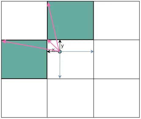
yolov5 正样本选取规则
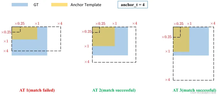
yolov5中正负样本的计算规则是:比较标注框和anchor的宽高,比例在0.25-4以内就是正样本。如下图所示:
gt的原本面积为蓝色,虚线标注了0.25倍和4倍。只要anchor在0.25-4之间,就是匹配成功。
如果存在标注框,则计算anchor和标注框的宽高比
if nt:
    # 获取宽高比
    r = t[..., 4:6] / anchors[:, None]

    # 获取 宽高比或宽高比倒数 中最大的一个,和4比较。self.hyp['anchor_t'] = 4
    j = torch.max(r, 1 / r).max(2)[0] < self.hyp['anchor_t']  # compare

    # 将正样本过滤出来
    t = t[j]  # filter
此时t保存的就是所有符合条件的标注框,后续用于计算anchor和网格信息。这一阶段的结束之后,输出的是所有符合条件的anchor。t保存的是 image, class, x, y, w, h,anchor_id,同一个图片会对应多个标注框,多个标注框可能会对应多个anchor。
跨anchor匹配
r计算的过程中包含了跨anchor匹配。在准备工作中已经介绍过将标注框复制了三份,每一份都分配了一个anchor,相当于一个标注框拥有三种不同大小的anchor。现在计算宽高比获得的结果只要符合条件的都会认为是正样本,3种anchor之间互不干扰,所以会出现一个标注框匹配多个anchor。
(Pdb) pp t.shape
torch.Size([3, 63, 7])
(Pdb) pp t
tensor([[[ 0.00000,  1.00000, 18.38171,  ...,  6.90862,  7.49398,  0.00000],
         [ 0.00000,  0.00000,  5.00814,  ...,  6.27480,  7.04943,  0.00000],
         [ 0.00000,  0.00000, 12.70904,  ...,  4.81701,  5.14418,  0.00000],
         ...,
         [ 5.00000,  0.00000, 10.32074,  ...,  5.19988,  5.59987,  0.00000],
         [ 5.00000,  0.00000, 31.28691,  ...,  5.79986,  6.66651,  0.00000],
         [ 5.00000,  0.00000, 51.81977,  ...,  5.66653,  5.93320,  0.00000]],

        [[ 0.00000,  1.00000, 18.38171,  ...,  6.90862,  7.49398,  1.00000],
         [ 0.00000,  0.00000,  5.00814,  ...,  6.27480,  7.04943,  1.00000],
         [ 0.00000,  0.00000, 12.70904,  ...,  4.81701,  5.14418,  1.00000],
         ...,
         [ 5.00000,  0.00000, 10.32074,  ...,  5.19988,  5.59987,  1.00000],
         [ 5.00000,  0.00000, 31.28691,  ...,  5.79986,  6.66651,  1.00000],
         [ 5.00000,  0.00000, 51.81977,  ...,  5.66653,  5.93320,  1.00000]],

        [[ 0.00000,  1.00000, 18.38171,  ...,  6.90862,  7.49398,  2.00000],
         [ 0.00000,  0.00000,  5.00814,  ...,  6.27480,  7.04943,  2.00000],
         [ 0.00000,  0.00000, 12.70904,  ...,  4.81701,  5.14418,  2.00000],
         ...,
         [ 5.00000,  0.00000, 10.32074,  ...,  5.19988,  5.59987,  2.00000],
         [ 5.00000,  0.00000, 31.28691,  ...,  5.79986,  6.66651,  2.00000],
         [ 5.00000,  0.00000, 51.81977,  ...,  5.66653,  5.93320,  2.00000]]], device='cuda:0')
(Pdb) pp t[0,0]
tensor([ 0.00000,  1.00000, 18.38171, 44.93684,  6.90862,  7.49398,  0.00000], device='cuda:0')
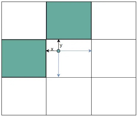
获取扩展网格
在yolov5中除了将gt中心点所在网格的anchor匹配为正样本之外,还会将网格相邻的上下左右四个网格中的对应anchor作为正样本。获取扩展网格的规则就是根据中心点距离上下左右哪个更近来确定扩展的网格。如下图中心点更靠近上和右,那么上和右网格中对应的anchor就会成为正样本。
获取扩展网格主要分为几步走:
- 获取所有gt的中心点坐标gxy
- 获取中心点坐标相对于右下边界的距离
- 计算中心点距离上下左右哪两个边界更近
- 获取所有anchor所在的网格,包括gt中心点所在网格和扩展网格
gxy = t[:, 2:4]  # grid xy
gxi = gain[[2, 3]] - gxy  # inverse
j, k = ((gxy % 1 < g) & (gxy > 1)).T
"""
(Pdb) ((gxy % 1 < g) & (gxy > 1)).shape
torch.Size([186, 2])
(Pdb) ((gxy % 1 < g) & (gxy > 1)).T.shape
torch.Size([2, 186])
"""
l, m = ((gxi % 1 < g) & (gxi > 1)).T

j = torch.stack((torch.ones_like(j), j, k, l, m))
"""
torch.ones_like(j) 代表gt中心所在grid cell
j, k, l, m 代表扩展的上下左右grid cell

torch.Size([5, 51])
"""
t = t.repeat((5, 1, 1))[j]
"""
标签也重复5次,和上面的扩展gird cell一起筛选出所有的,符合条件的grid cell
(Pdb) pp t.shape
torch.Size([153, 7])
(Pdb) t.repeat((5, 1, 1)).shape
torch.Size([5, 153, 7])
(Pdb) pp t.shape
torch.Size([232, 7])
"""
offsets = (torch.zeros_like(gxy)[None] + off[:, None])[j]
"""
计算出所有grid cell的偏移量,作用在标签上之后就能得到最终的grid cell
(Pdb) pp offsets.shape
torch.Size([529, 2])
"""
gxy 是中心点的坐标,中心点坐标是相对于整个80*80网格的左上角(0,0)的距离,而gxi是80减去中心点坐标,得到的结果相当于是中心点距离(80,80)的距离。将中心点取余1之后相当于缩放到一个网格中,如上图所示。
gxy = t[:, 2:4]  # grid xy
gxi = gain[[2, 3]] - gxy  # inverse
j, k = ((gxy % 1 < g) & (gxy > 1)).T
模拟以上操作,j,k得到的是一组布尔值
>>> import torch
>>>
>>> arr = torch.tensor([[1,2,3], [4,5,6]])
>>> one = arr % 2 < 2
>>> two = arr > 3
>>> one
tensor([[True, True, True],
        [True, True, True]])
>>> two
tensor([[False, False, False],
        [ True,  True,  True]])
>>> one & two
tensor([[False, False, False],
        [ True,  True,  True]])
距离的计算过程:
j, k = ((gxy % 1 < g) & (gxy > 1)).T
"""
(Pdb) ((gxy % 1 < g) & (gxy > 1)).shape
torch.Size([186, 2])
(Pdb) ((gxy % 1 < g) & (gxy > 1)).T.shape
torch.Size([2, 186])
"""
l, m = ((gxi % 1 < g) & (gxi > 1)).T
gxy % 1 < g 代表x或y离左上角距离小于0.5,小于0.5也就意味着靠的更近
gxy > 1 代表x或y必须大于1,x必须大于1也就是说第一行的网格不能向上扩展;y必须大于1就是说第一列的网格不能向左扩展。
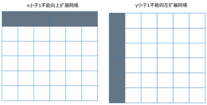
同理gxi是相对下边和右边的距离,得到布尔张量。
l, m = ((gxi % 1 < g) & (gxi > 1)).T
获取所有的正样本网格结果
j = torch.stack((torch.ones_like(j), j, k, l, m))
t = t.repeat((5, 1, 1))[j]
j 保存上面扩展网格和中心点网格的匹配结果,是bool数组。torch.ones_like(j) 表示中心点匹配到的网格,jklm中保存的上下左右匹配的网格。
t是将gt中心点的网格复制出来5份,用于计算所有网格。第一份是中心点匹配结果,剩余四份是上下左右网格匹配结果。
用j来筛选t,最终留下所有选中的网格。
计算出从中心点网格出发到扩展网格的需要的偏移量。后续使用使用该偏移量即可获取所有网格,包括中心点网格和扩展网格。计算的过程中涉及到了广播机制。
offsets = (torch.zeros_like(gxy)[None] + off[:, None])[j]
示例如下:
>>> off
tensor([[ 0,  0],
        [ 1,  0],
        [ 0,  1],
        [-1,  0],
        [ 0, -1]])
>>> arr = torch.tensor([10])
>>>
>>>
>>> arr + off
tensor([[10, 10],
        [11, 10],
        [10, 11],
        [ 9, 10],
        [10,  9]])
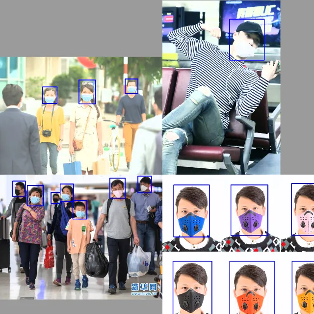
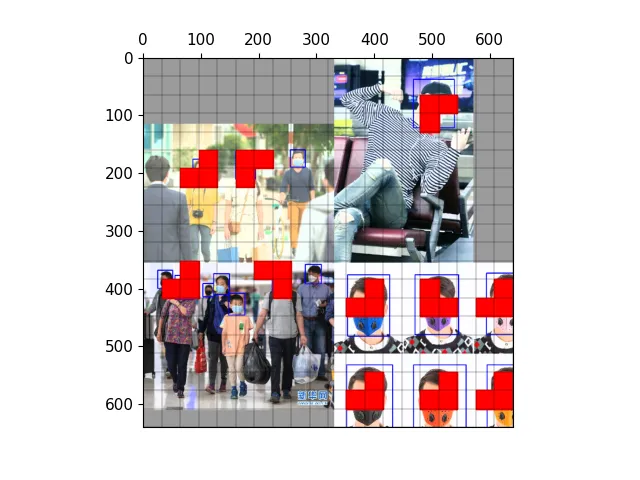
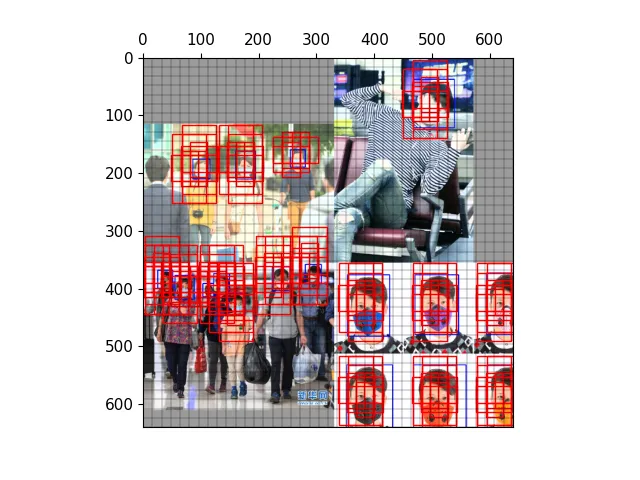
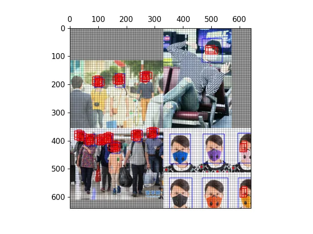
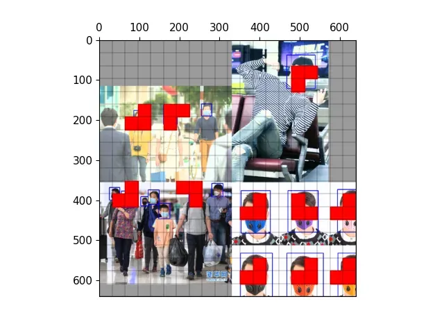
以下图为例,可视化正样本anchor。
经过mosaic处理的图片,蓝色为标注框
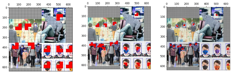
三种尺度下的正样本网格
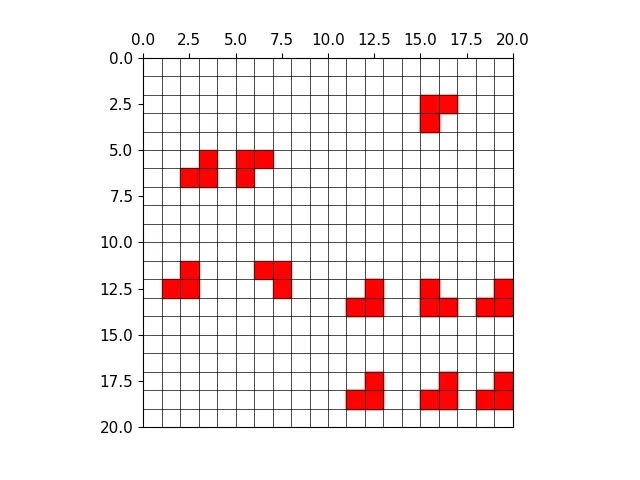
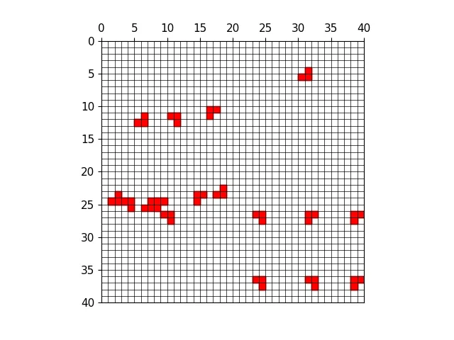
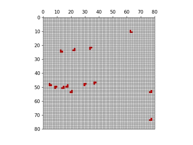
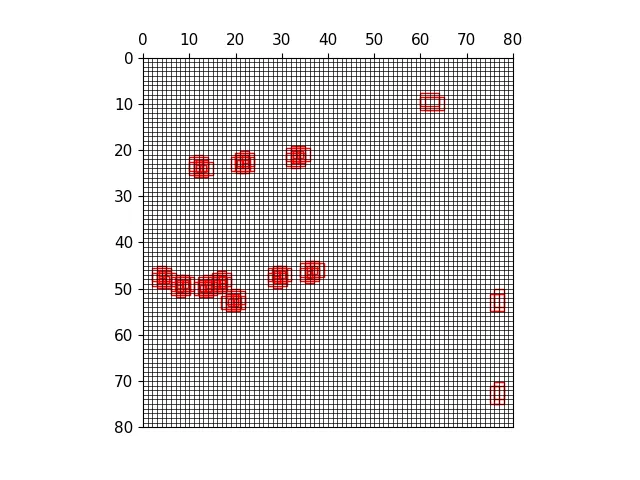
三种尺度下的正样本anchor
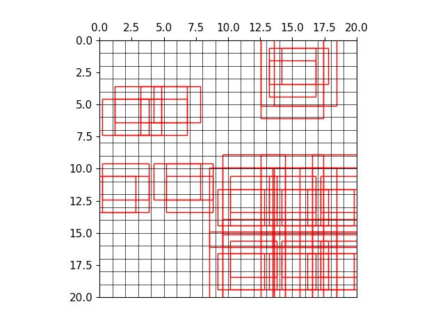
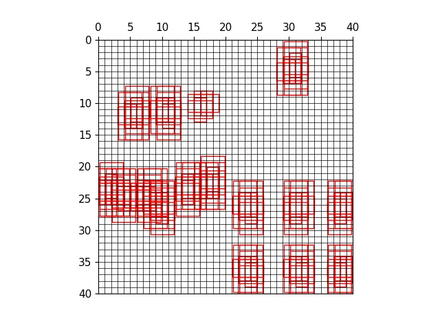
三种尺度下原图的正样本网格
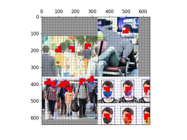
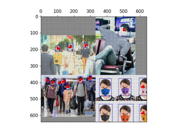
三种尺度下原图的anchor
保存结果
从t中获取相关数据,包括:
- bc:image_id, class_id
- gxy: gt中心点坐标
- gwh: gt宽高
- a: anchor_id
bc, gxy, gwh, a = t.chunk(4, 1)  # (image, class), grid xy, grid wh, anchors
a, (b, c) = a.long().view(-1), bc.long().T  # anchors, image, class
gij = (gxy - offsets).long()
获取所有正样本网格:
gij = (gxy - offsets).long()
gi, gj = gij.T  # grid indices
gxy是gt中心点的坐标,减去对应偏移量再取整, 得到所有正样本所在网格。然后将xy拆分出来得到gi,gj。
(Pdb) pp gij
tensor([[74, 24],
        [37, 28],
        [72,  9],
        [75, 11],
        [67,  5],
        [73,  5],
        [70,  5],
        [75,  1],
        ...)
indices: 保存图片,anchor,网格等信息
# indices 保存的内容是:image_id, anchor_id(0,1,2), grid x刻度  grid y刻度。这里的刻度就是正样本
indices.append((b, a, gj.clamp_(0, shape[2] - 1), gi.clamp_(0, shape[3] - 1)))  # image, anchor, grid
(Pdb) pp a.shape
torch.Size([367])
(Pdb) pp gij.shape
torch.Size([367, 2])
保存中心点偏移量
# tbox保存的是gt中心相对于所在grid cell左上角偏移量。也会计算出gt中心相对扩展anchor的偏移量
tbox.append(torch.cat((gxy - gij, gwh), 1))  # box
gij是网格起始坐标,gxy是gt中心点坐标。gxy-gij就是获取gt中心点相对于网格左上角坐标的偏移量。
在后续的损失函数计算中,用这个偏移量和网络预测出来的偏移量计算损失函数。
保存anchor具体的宽高和类别id
anch.append(anchors[a])  # anchors # 保存anchor的具体宽高
tcls.append(c)  # class 保存类别id
自此正样本筛选的流程就结束了,最终返回了4个张量:
- indices 保存的内容是:image_id, anchor_id, grid x刻度 grid y刻度
- tbox 保存的是gt中心相对于所在grid cell左上角偏移量。也会计算出gt中心相对扩展anchor的偏移量
- anchors 保存anchor的具体宽高
- class 保存类别id
返回的正样本anchor会在后续损失函数的计算中使用。用 indices 保存的网格筛选出模型输出的中对应的网格里的内容,用tbox中中心点相对网格的偏移和模型输出的预测中心点相对于网格左上角偏移量计算偏差,并不断修正。
Q&A
一、正样本指的是anchor,anchor匹配如何体现在过程?
targets 是这一批图片的标注信息,每一行的内容分别是:image, class, x, y, w, h。
(Pdb) pp targets.shape
torch.Size([63, 6])

tensor([[0.00000, 1.00000, 0.22977, 0.56171, 0.08636, 0.09367],
        [0.00000, 0.00000, 0.06260, 0.59307, 0.07843, 0.08812],
        [0.00000, 0.00000, 0.15886, 0.59386, 0.06021, 0.06430],
        [0.00000, 0.00000, 0.31930, 0.58910, 0.06576, 0.09129],
        [0.00000, 0.00000, 0.80959, 0.70458, 0.23025, 0.26275],
        [1.00000, 1.00000, 0.85008, 0.07597, 0.09781, 0.11827],
        [1.00000, 0.00000, 0.22484, 0.09267, 0.14065, 0.18534]
targets = torch.cat((targets.repeat(na, 1, 1), ai[..., None]), 2)
>>>
(Pdb) pp targets.shape
torch.Size([3, 63, 7])
targets保存的标注信息,首先将标注信息复制成三份,因为每一个尺度每一个网格上有三个anchor,相当于给一份标注框分配了一个anchor。
在后续的操作中,先通过先将标注框还原到对应的尺度上,通过宽高比筛选anchor,获得符合正样本的anchor。到这里就获得所有正样本的anchor。
然后再通过中心点的坐标获得扩展网格。
j = torch.stack((torch.ones_like(j), j, k, l, m))
t = t.repeat((5, 1, 1))[j]
此时将t复制5份,每一份的每一行内容代表:image, class, x, y, w, h,anchor_id。
复制的过程中就携带了anchor_id的信息,最终通过扩展获取上下左右两个网格,相当于获得了两个网格中的anchor。
最后将所有的anchor保存起来,在计算损失函数时使用到anchor的两个功能:
- 使用这些anchor的宽高作为基准,模型输出的结果是anchor宽高的比例
- anchor所在的网格为定位参数提供范围。网络输出的xy是相对于网格左上角的偏移
二、 跨anchor匹配体现在哪里?
targets保存的标注信息,首先将标注信息复制成三份,因为每一个尺度每一个网格上有三个anchor,相当于给一份标注框分配了一个anchor。
r = t[..., 4:6] / anchors[:, None]

# 获取 宽高比或宽高比倒数 中最大的一个,和0.5比较
j = torch.max(r, 1 / r).max(2)[0] < self.hyp['anchor_t']  # compare

# 将正样本过滤出来
t = t[j]  # filter
r计算的过程中包含了跨anchor匹配。t是将原有的标注信息复制了三份,而每一个网格也有三个anchor,也就是说一份标注信息对应一个anchor。现在计算宽高比获得的结果只要符合条件的都会认为是正样本,3种anchor之间互不干扰。
那么有可能存在的情况是三种anchor和gt的宽高比都符合条件,那么这3个标注数据都会保存下来,相应的anchor都会成为正样本。
三、跨网格匹配体现在哪里?
所谓跨网格匹配就是除了gt中心点所在网格,还会选择扩展网格。
扩展网格的筛选过程就是跨网格匹配的过程
gxy = t[:, 2:4]  # grid xy
gxi = gain[[2, 3]] - gxy  # inverse
j, k = ((gxy % 1 < g) & (gxy > 1)).T
l, m = ((gxi % 1 < g) & (gxi > 1)).T
j = torch.stack((torch.ones_like(j), j, k, l, m))
t = t.repeat((5, 1, 1))[j]
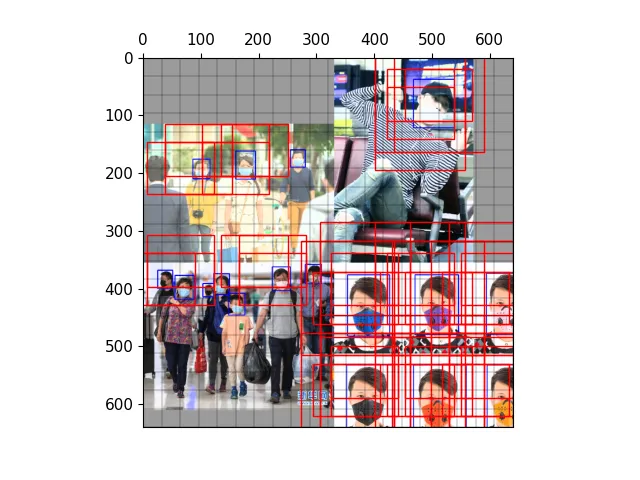
四、跨尺度匹配体现在哪里?
一个标注框可以在不同的预测分支上匹配上anchor。anchor的匹配在不同的尺度上分开单独处理,三个尺度互相不干扰,所以一个标注框最多能在三个尺度上都匹配上anchor。
for i in range(self.nl):
    anchors, shape = self.anchors[i], p[i].shape
    ...
    indices.append((b, a, gj.clamp_(0, shape[2] - 1), gi.clamp_(0, shape[3] - 1)))  # image, anchor, grid

    # tbox保存的是gt中心相对于所在grid cell左上角偏移量。也会计算出gt中心相对扩展anchor的偏移量
    tbox.append(torch.cat((gxy - gij, gwh), 1))  # box
可以看到以下三个不同尺度的anchor匹配中,右上角目标都匹配上了。
五、扩展的网格中用哪一个anchor?
通过宽高比筛选出来的正样本才会被复制,也就是说一个网格中的anchor匹配上gt之后,然后才有可能被扩展网格选中。
在扩展网格之前,就已经筛选出正样本,有一个确定大小的anchor。扩展网格的获得过程是将正样本复制5份。复制的过程就将中心点匹配的anchor_id携带过去。
j = torch.stack((torch.ones_like(j), j, k, l, m))
t = t.repeat((5, 1, 1))[j]
复制的是正样本,那么扩展网格最终获得的也是中心点所在网格上匹配好的anchor
一个网格中有两个anchor成为正样本,那么扩展网格中就有两个anchor为正样本。扩展网格的anchor_id 和中心点网格保持一致。
六、扩展网格中gt的偏移量如何计算?
计算gt中心点相对于网格左上角的偏移量中有几个变量:
- gxy: 中心点的坐标
- gij:网格的起始坐标
gij = (gxy - offsets).long()
gij 是通过中心点减去偏移量再取整获得的
# tbox保存的是gt中心相对于所在grid cell左上角偏移量。也会计算出gt中心相对扩展anchor的偏移量
tbox.append(torch.cat((gxy - gij, gwh), 1))  # box
gxy - gij 的计算过程中,对于那些扩展的网格,也会同样计算偏移量。所以扩展网格的偏移量就是网格的左上角到gt中心点的距离。

 浙公网安备 33010602011771号