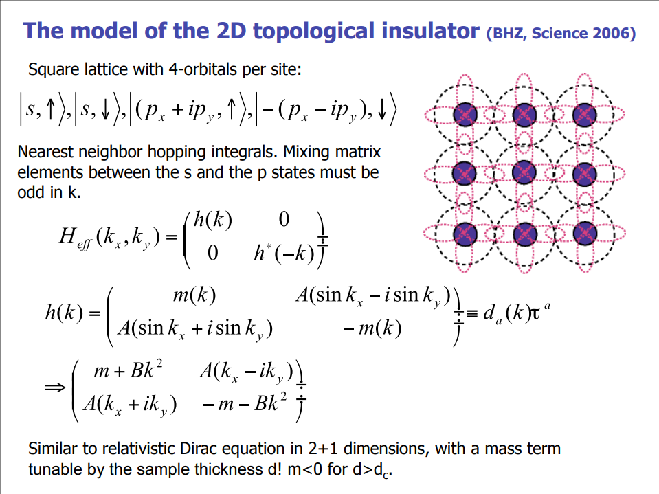
BHZ Model Hamiltonian
HgTe 量子阱
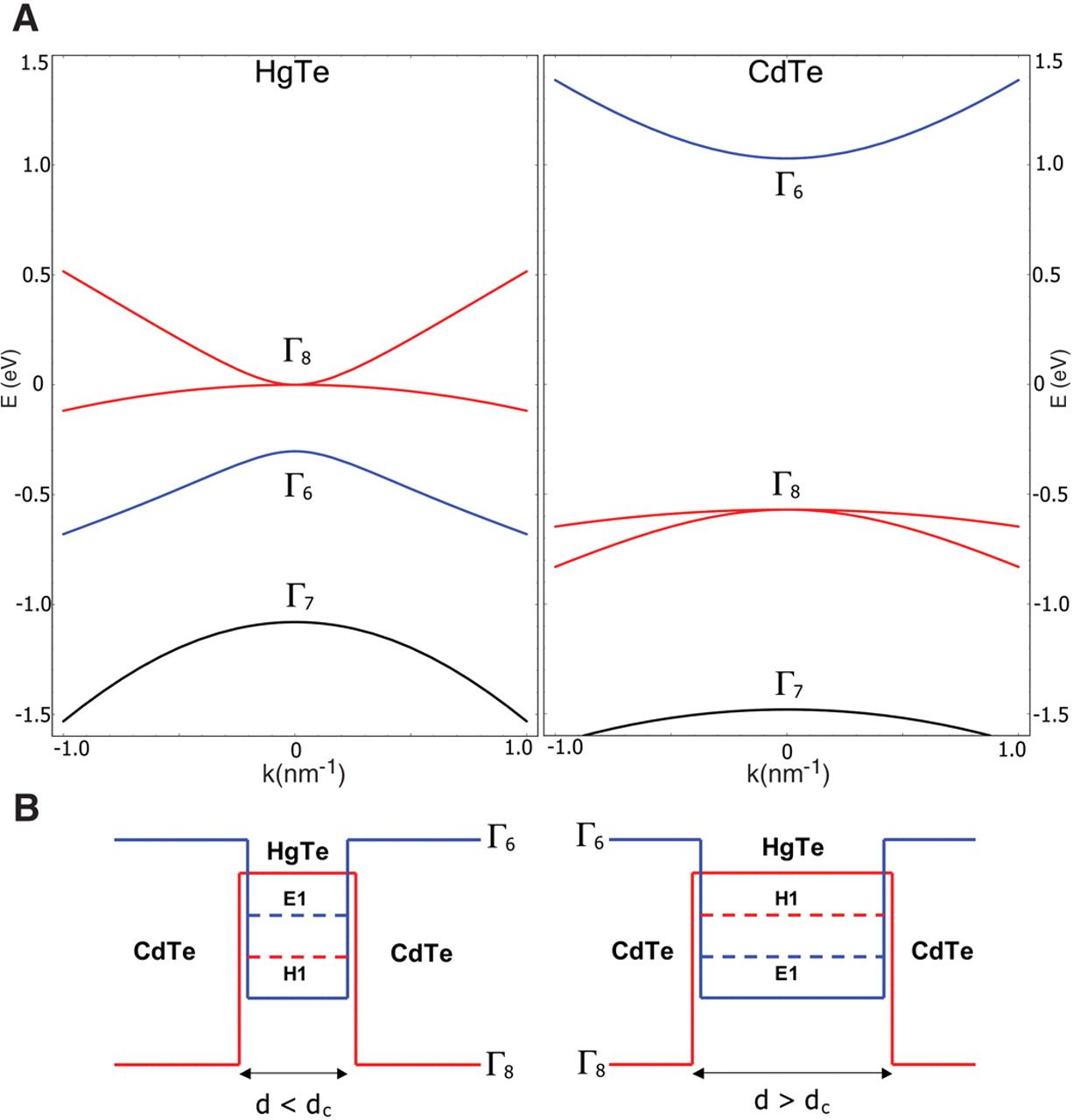
CdTe 和 HgTe 的晶格结构类似,属于闪锌矿结构,点群是 \(T_d\)。如图所示,从能带上看 CdTe 的能带与常见的半导体能带一致,\(\Gamma_6 (s)\) 带在 \(\Gamma_8 (p)\) 带之上,\(\Gamma_7\) 为自旋轨道劈裂带。然而 HgTe 的能带结构却是反常的,\(\Gamma_8\) 带在 \(\Gamma_6\) 之上。HgTe 表现出半金属性的电子性质。因此,把 CdTe 和 HgTe 制作成一个异质结,来调控 HgTe 的能带结构。
 量子阱色散关系
当 \(d > d_c\), 能带出现反转,进入量子自旋霍尔态。
当 \(d < d_c\),为常规的绝缘态。
哈密顿量基矢
对于常见的半导体费米面附近的能带,通过用 Kane 八带模型去描述。由于 \(\Gamma_7\) 离 \(\Gamma_{6,8}\) 较远,忽略它的影响,选择以 \(\Gamma_6,\Gamma_8\) 为基矢的六带模型。基矢如下:
在 [001] 方向生长的量子阱中,立方对称性破缺到一个 \(C_{4z}\) 的对称性,这六个带重新组合为自旋上下 \(E1,H1,L1\)带。费米面附近有效的四带模型哈密顿量来自 \(E1,H1\)。\(|E1,\pm\frac{1}{2}\rangle\) 来自于 \(|\Gamma_6,\pm\frac{1}{2}\rangle\) 和 \(|\Gamma_8,\pm\frac{1}{2}\rangle\) 的线性组合。\(|H1,\pm\frac{1}{2}\rangle\) 来自于\(|\Gamma_8,\pm\frac{3}{2}\rangle\).
对称性
费米面附近的轨道为 \(E1+, H1+, E1-, H1-\)。
The symmetry group is generated by spatial inversion symmetry \(P\), time-reversal symmetry \(T\) and fourfold rotation symmetry \(C_{4z}\).
为了简单地说明问题,直接选用 Science 318, 766-770(2007) 里面的基矢:
空间反演
对于空间反演 \(P\): (x,y,z) -> (-x,-y,-z):
表示矩阵为
时间反演
对于时间反演 \(T\): \(T=i\sigma_y K\):
表示矩阵为
四度旋转对称
对于四度旋转对称性 \(C_{4z}\): (x,y,z) -> (-y,x,z):
先介绍一下自旋旋转矩阵 (参考自旋旋转矩阵):
因此,\(C_{4z}\) 作用在自旋上为: \(C_{4z}|\uparrow\rangle=e^{-i\pi/4}|\uparrow\rangle, C_{4z}|\downarrow\rangle=e^{i\pi/4}|\downarrow\rangle\)。
因此,
表示矩阵为
运行 Qsymm 程序得到 \(k\cdot p\) 哈密顿量得到:
Matrix([[1, 0, 0, 0], [0, 0, 0, 0], [0, 0, 1, 0], [0, 0, 0, 0]])
Matrix([[0, 0, 0, 0], [0, 1, 0, 0], [0, 0, 0, 0], [0, 0, 0, 1]])
Matrix([[k_x**2 + k_y**2, 0, 0, 0], [0, 0, 0, 0], [0, 0, k_x**2 + k_y**2, 0], [0, 0, 0, 0]])
Matrix([[0, 0, 0, 0], [0, k_x**2 + k_y**2, 0, 0], [0, 0, 0, 0], [0, 0, 0, k_x**2 + k_y**2]])
猜测
如果基矢选为:
空间反演对称性表示矩阵为:
时间反演对称性表示矩阵为
四度旋转表示矩阵为
最后可得到文献里的哈密顿量。
问题
Time Reversal for Spin-\(\frac{3}{2}\) : Find a representation for the TR operator for spin--\(\frac{3}{2}\) particles.
附录
Qsymm 运行代码
点击查看代码
import numpy as np
import sympy
import qsymm

# Spatial inversion
pU = np.array([
    [1.0, 0.0, 0.0, 0.0],
    [0.0, -1.0, 0.0, 0.0],
    [0.0, 0.0, 1.0, 0.0],
    [0.0, 0.0, 0.0, -1.0],
])
pS = qsymm.inversion(2, U=pU)

# Time reversal
trU = np.array([
    [0.0, 0.0, -1.0, 0.0],
    [0.0, 0.0, 0.0, 1.0],
    [1.0, 0.0, 0.0, 0.0],
    [0.0, -1.0, 0.0, 0.0],
])
trS = qsymm.time_reversal(2, U=trU)

# Rotation
phi = 2.0 * np.pi / 4.0  # Impose 4-fold rotational symmetry
rotU = np.array([
    [np.exp(-1j*phi/2), 0.0, 0.0, 0.0],
    [0.0, np.exp(1j*1*phi/2), 0.0, 0.0],
    [0.0, 0.0, np.exp(1j*phi/2), 0.0],
    [0.0, 0.0, 0.0, np.exp(1j*3*phi/2)],
])
rotS = qsymm.rotation(1/4, U=rotU)

symmetries = [rotS, trS, pS]
# print(symmetries)
dim = 2
total_power = 2

family = qsymm.continuum_hamiltonian(symmetries, dim, total_power, prettify=True)
qsymm.display_family(family)
Qsymm 运行代码2
点击查看代码
import numpy as np
import sympy
import qsymm

# Spatial inversion
pU = np.array([
    [1.0, 0.0, 0.0, 0.0],
    [0.0, -1.0, 0.0, 0.0],
    [0.0, 0.0, 1.0, 0.0],
    [0.0, 0.0, 0.0, -1.0],
])
pS = qsymm.inversion(2, U=pU)

# Time reversal
trU = np.array([
    [0.0, 0.0, -1.0, 0.0],
    [0.0, 0.0, 0.0, -1.0],
    [1.0, 0.0, 0.0, 0.0],
    [0.0, 1.0, 0.0, 0.0],
])
trS = qsymm.time_reversal(2, U=trU)

# Rotation
phi = 2.0 * np.pi / 4.0  # Impose 4-fold rotational symmetry
rotU = np.array([
    [np.exp(-1j*phi/2), 0.0, 0.0, 0.0],
    [0.0, np.exp(-1j*3*phi/2), 0.0, 0.0],
    [0.0, 0.0, np.exp(1j*phi/2), 0.0],
    [0.0, 0.0, 0.0, np.exp(1j*3*phi/2)],
])
rotS = qsymm.rotation(1/4, U=rotU)

symmetries = [rotS, trS, pS]
# print(symmetries)
dim = 2
total_power = 2

family = qsymm.continuum_hamiltonian(symmetries, dim, total_power, prettify=True)
qsymm.display_family(family)

### Output
'''
Matrix([[1, 0, 0, 0], [0, 0, 0, 0], [0, 0, 1, 0], [0, 0, 0, 0]])
Matrix([[0, 0, 0, 0], [0, 1, 0, 0], [0, 0, 0, 0], [0, 0, 0, 1]])
Matrix([[0, k_x + I*k_y, 0, 0], [k_x - I*k_y, 0, 0, 0], [0, 0, 0, -k_x + I*k_y], [0, 0, -k_x - I*k_y, 0]])
Matrix([[0, I*k_x - k_y, 0, 0], [-I*k_x - k_y, 0, 0, 0], [0, 0, 0, I*k_x + k_y], [0, 0, -I*k_x + k_y, 0]])
Matrix([[k_x**2 + k_y**2, 0, 0, 0], [0, 0, 0, 0], [0, 0, k_x**2 + k_y**2, 0], [0, 0, 0, 0]])
Matrix([[0, 0, 0, 0], [0, k_x**2 + k_y**2, 0, 0], [0, 0, 0, 0], [0, 0, 0, k_x**2 + k_y**2]])
'''

 浙公网安备 33010602011771号