A self-consistent solution of Schrodinger-Poisson equations

Poisson Equations

The fundamental equations in electromagnetism is

$$\hat{\bm E} = -\nabla \phi\\ \nabla\cdot \hat{\bm D} = \rho \rightarrow \nabla\cdot \varepsilon_r\hat{\bm E} = \frac{\rho}{\varepsilon_0} \tag{1.1}$$

combinated the two equations, then we obtain

$$\varepsilon_r\nabla^2\phi(r) = -\frac{\rho(r)}{\varepsilon_0}. \tag{1.2}$$

where $\varepsilon_r$ is the dielectric constant, $\phi$ is the electrostatic potential. More specifically,

$$-\varepsilon_r\nabla^2\phi(r) = \frac{\rho(r)}{\varepsilon_0} =\frac{q((N_d^{+}(r)-n(r)-N_a^{-}(r)+p(r))}{\varepsilon_0}. \tag{1.3}$$

where $N_d,N_a$ denote the ionized donor and acceptor densities, $n,p$ denote the electron and hole densities, these quantities are positive.

Basic Equations

The one-dimensional, one-electron schrodinger equation is

$$-\frac{\hbar^2}{2}\frac{d}{dx}(\frac{1}{m^*(x)}\frac{d}{dx})\psi(x) + V(x)\psi(x) = E\psi(x). \tag{2.1}$$

where $\psi$ is the wave function, $E$ is the energy, $V$ is the potential energy, $\hbar$ is Plack's constant divided by $2\pi$, and $m^*$ is the effective mass.

For a simple $n$-type materilas, the one-dimensional Poisson equation is

$$\frac{d}{dx}\left(\varepsilon_r(x)\frac{d}{dx}\right)\phi(x) = \frac{-q(N_d(x)-n(x))}{\varepsilon_0}, \tag{2.2}$$

To find the electron distribution in the condution band, one may set the potential energy $V$ to be equal to the conduction-band energy. In a quantum well of arbitrary potential energy profile, the potential energy $V$ is related to the electrostatic potential $\phi$ as follows:

$$V(x) = -q\phi(x) + \Delta E_c(x), \tag{2.3}$$

where $\Delta E_c(x)$ is the pseudopotential energy due to the band offset at the heterointerface. The wave function $\psi$ and the electron density are related by

$$n(x) = \sum_{k=1}^{m}\psi_k^*(x)\psi_k(x)f_k \tag{2.4}$$

where $m$ is the number of bound states, and $f_k$ is the electron occupation for each state. The electron concentration for each state are be expressed by

$$f_k = \frac{m^*}{\pi\hbar^2}\int^{\infty}_{E_k}\frac{1}{1+e^{(E-E_f)/kT}}dE. \tag{2.5}$$

where $E_k$ is the eigenenergy.

Newton's method

Since the electron density is determined by solutions of the schrodinger equation which are in turn determined by the potential $\phi(x)$, the electron density is actually a functional by $n[\phi]$. The one dimensional Poisson's equation can be written as

$$\frac{d}{dx}\left(\varepsilon_r\frac{d\phi}{dx}\right) = \frac{-q(N_d-n[\phi])}{\varepsilon_0}. \tag{3.1}$$

Let us denote the exact solution by $\phi^0(x)$. For a given trial function $\phi(x)$ (or the initial guess), our task is to find the correction $\delta\phi(x)$ so that

$$\phi^0(x) = \phi(x) + \delta\phi(x). \tag{3.2}$$

Then, we obtain

$$\frac{d}{dx}\left(\varepsilon_r\frac{d\phi}{dx}\right) = \frac{-q(N_d-n[\phi+\delta\phi])}{\varepsilon_0}-\frac{d}{dx}\left(\varepsilon_r\frac{d\delta\phi}{dx}\right). \tag{3.3}$$

Defining: $n[\phi+\delta\phi] = n[\phi] + \delta n[\phi]$, then

$$-\left[\frac{d}{dx}\left(\varepsilon_r\frac{d\phi}{dx}\right)+\frac{q(N_d-n[\phi])}{\varepsilon_0}\right]= \frac{d}{dx}\left(\varepsilon_r\frac{d\delta\phi}{dx}\right)-\frac{q}{\varepsilon_0}\delta n[\phi]. \tag{3.4}$$

Note that the left-band side is the error in Poisson's equation for the trivial function $\phi(x)$ which can be easily calculated. Assuming the $\delta\phi(x)$ is small, from (2.4) and (3.4), $\delta n[\phi]$ can be expressed as

$$\delta n[\phi] = \sum_{k=1}^m[\delta(\psi_{k}^*\psi_k)f_k + \psi_{k}^*\psi_k\delta f_k] \tag{3.5}$$

where

$$\delta(\psi_{k}^*\psi_k) = \psi_k^*[\phi+\delta\phi]\psi_k[\phi+\delta\phi]-\psi_k^*[\phi]\psi_k[\phi]\\ \delta n_k=n_k(\phi+\delta\phi) - n_k(\phi) \tag{3.6}$$

THe relevant numerical experience indicates that the first term on the right-hand side of Eq.(3.5) is usually much smaller than the second one. Dropping the first term and expressing $\delta n_k$ in terms of $\delta\phi$.

$$\delta n(\phi)=-\frac{m^*}{\pi\hbar^2}\sum_{k=1}^{m}\psi_k\psi_k\frac{1}{1+e^{(E_k-E_f)/kT}}\cdot <\psi_k|q\delta\phi|\psi_k>$$

Therefore,

$$-\left[\frac{d}{dx}\left(\varepsilon_r\frac{d\phi}{dx}\right)+\frac{q(N_d-n)}{\varepsilon_0}\right]= \frac{d}{dx}\left(\varepsilon_r\frac{d\delta\phi}{dx}\right)+\frac{q}{\varepsilon_0}\sum_{k=1}^{m}\psi_k^*\psi_k\frac{\partial n_k}{\partial E_k}\cdot <\psi_k|q\delta\phi|\psi_k>. \tag{3.8}$$

$$\delta n[\phi] = \frac{dn}{d\phi}\delta\phi$$

For the typical quantum transport,

$$n = 2*f_{3D}(E_c+U(r)-\mu)\\ f_{3D}(E) = \left(\frac{m_ck_BT}{2\pi\hbar^2}\right)^{3/2}\Im_{1/2}(-\frac{E}{k_BT})=N_c\Im_{1/2}(-\frac{E}{k_BT}).\\ \Im_{1/2}(x)=\frac{2}{\sqrt{\pi}}\int^{\infty}_0\frac{d\xi\sqrt{\xi}}{1+exp(\xi-x)}$$

Final, we can get

$$\frac{dn}{d\phi} = 2N_c\frac{d\Im}{d\phi}\frac{q}{k_BT}.$$

$$\frac{d^2}{dx^2}U-\frac{q^2(N_D-n[U])}{\varepsilon_0\varepsilon_s}= -\frac{d^2}{dx^2}\delta U-\frac{q^2}{\varepsilon_0\varepsilon_s}\frac{dn}{dU}\delta U.$$

$$D_2U-\beta(N_D-n)= -(D_2+\beta\frac{dn}{dU})\delta U.$$

$$\beta^{-1} D_2U-(N_D-n)= -\beta^{-1}(D_2+\beta\frac{dn}{dU})\delta U.$$

$$\delta U = -\beta(D_2+\beta\frac{dn}{dU})^{-1}*(\beta^{-1} D_2U-N_D+n).$$

Matlab Code

The code is copied from the Supriyo Datta's textbook.

点击查看代码

%Fig.3.1 
clear all 
  
%Constants (all MKS, except energy which is in eV) 
hbar=1.06e-34;q=1.6e-19;epsil=10*8.85E-12;kT=.025; m=.25*9.1e-31;
n0=2*m*kT*q/(2*pi*(hbar^2)); 
  
%inputs 
a=3e-10;t=(hbar^2)/(2*m*(a^2)*q);beta=q*a*a/epsil; 
Ns=15;Nc=70;Np=Ns+Nc+Ns;XX=a*1e9*[1:1:Np]; 
mu=.318;Fn=mu*ones(Np,1); 
Nd=2*((n0/2)^1.5)*Fhalf(mu/kT) 
Nd=Nd*[ones(Ns,1);.5*ones(Nc,1);ones(Ns,1)]; 
  
%d2/dx2 matrix for Poisson solution 
D2=-(2*diag(ones(1,Np)))+(diag(ones(1,Np-1),1))+...
(diag(ones(1,Np-1),-1)); 
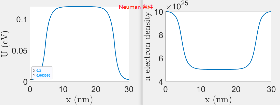
%D2(1,1)=-1;D2(Np,Np)=-1;%zero field condition 
  
%Hamiltonian matrix 
T=(2*t*diag(ones(1,Np)))-(t*diag(ones(1,Np-1),1))-(t*diag(ones(1,Np-1),-1)); 
  
%energy grid 
NE=501;E=linspace(-.25,.5,NE);dE=E(2)-E(1);zplus=1i*1e-20; 
f0=n0*log(1+exp((mu-E)./kT)); 
  
%self-consistent calculation 
U=[zeros(Ns,1);.2*ones(Nc,1);zeros(Ns,1)];%guess for U 

dU=0;ind=10; 
while ind>0.001
    %from U to n 
    sig1=zeros(Np);sig2=zeros(Np);n=zeros(Np,1); 
    for k=1:NE 
        ck=1-((E(k)+zplus-U(1))/(2*t));ka=acos(ck); 
        sig1(1,1)=-t*exp(1i*ka);gam1=1i*(sig1-sig1'); 
        ck=1-((E(k)+zplus-U(Np))/(2*t));ka=acos(ck); 
        sig2(Np,Np)=-t*exp(1i*ka);gam2=1i*(sig2-sig2'); 
        G=inv(((E(k)+zplus)*eye(Np))-T-diag(U)-sig1-sig2); 
        A=1i*(G-G');rhoE=f0(k)*diag(A)./(2*pi); 
        n=n+((dE/a)*real(rhoE)); 
    end
    
    %correction dU from Poisson
    D=zeros(Np,1); 
    for k=1:Np 
        z=(Fn(k)+U(k))/kT; 
        D(k)=2*((n0/2)^1.5)*((Fhalf(z+.1)-Fhalf(z))/.1)/kT; 
    end
    
    dN=n-Nd+((1/beta)*D2*U);
    dU=(-beta)*(inv(D2-(beta*diag(D))))*dN;U=U+dU; 
    
    %check for convergence 
    ind=(max(max(abs(dN))))/(max(max(Nd))) 

end 
%plot(XX,n) 
%plot(XX,U) 
%plot(XX,F,':') 

save fig31 

figure
hold on
h=plot(XX,U);
grid on
set(h,'linewidth',[2.0])
set(gca,'Fontsize',[24])
xlabel(' x (nm)', 'Interpreter', 'latex')
ylabel('U (eV)', 'Interpreter', 'latex')


figure
hold on
h=plot(XX,n);
grid on
set(h,'linewidth',[2.0])
set(gca,'Fontsize',[24])
xlabel(' x (nm)', 'Interpreter', 'latex')
ylabel('n electron density', 'Interpreter', 'latex')

%For periodic boundary conditions, add 
 %           T(1,Np)=-t;T(Np,1)=-t; 
%and replace section entitled "from U to n" with 
            %from U to n 
            %[P,D]=eig(T+diag(U));D=diag(D); 
            %rho=log(1+exp((Fn-D)./kT));rho=P*diag(rho)*P'; 
            %n=n0*diag(rho);n=n./a; 

点击查看代码(Direclet边界条件)

clear all
tic

%Constants (all MKS, except energy which is in eV)
hbar=1.06e-34;q=1.6e-19;epsil=10*8.85E-12;kT=.025;
m=.25*9.1e-31;n0=2*m*kT*q/(2*pi*(hbar^2));

%inputs
a=3e-10;t=(hbar^2)/(2*m*(a^2)*q);beta=q*a*a/epsil;
Ns=15;Nc=70;Np=Ns+Nc+Ns;XX=a*1e9*[1:1:Np];
mu=.318;Fn=mu*ones(Np,1);
Nd=2*((n0/2)^1.5)*Fhalf(mu/kT);
Nd=Nd*[ones(Ns,1);0.5*ones(Nc,1);ones(Ns,1)];
%Nd=zeros(Np,1);

%d2/dx2 matrix for Poisson solution
D2=-(2*diag(ones(1,Np)))+(diag(ones(1,Np-1),1))+(diag(ones(1,Np-1),-1));
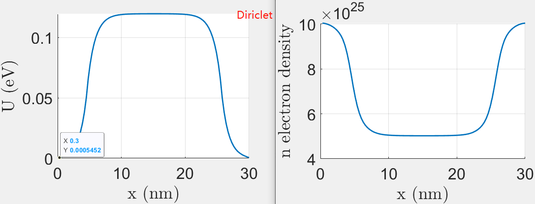
% D2(1,1)=-1;D2(Np,Np)=-1;%zero field condition
iD2 = inv(D2);
U0 = iD2*[0;zeros(Np-2,1);0];
%U0 = iD2*zeros(Np,1);

%Hamiltonian matrix
T=(2*t*diag(ones(1,Np)))-(t*diag(ones(1,Np-1),1))-(t*diag(ones(1,Np-1),-1));

%energy grid
NE=301;E=linspace(-.25,.5,NE);dE=E(2)-E(1);zplus=1i*1e-12;
f0=n0*log(1+exp((mu-E)./kT));

%self-consistent calculation
U=[zeros(Ns,1);.2*ones(Nc,1);zeros(Ns,1)];%guess for U

ind=10;
while ind>0.01
    %from U to n
    sig1=zeros(Np);sig2=zeros(Np);n=zeros(Np,1);
    for k=1:NE
        sig1=zeros(Np);sig2=zeros(Np);
        ck=1-((E(k)+zplus-U(1))/(2*t));ka=acos(ck);
        sig1(1,1)=-t*exp(1i*ka);gam1=1i*(sig1-sig1');
        ck=1-((E(k)+zplus-U(Np))/(2*t));ka=acos(ck);
        sig2(Np,Np)=-t*exp(1i*ka);gam2=1i*(sig2-sig2');
        
        G=inv(((E(k)+zplus)*eye(Np))-T-diag(U)-sig1-sig2);
        A=1i*(G-G');rhoE=f0(k)*diag(A)./(2*pi);
        n=n+((dE/a)*real(rhoE));
    end
    
    UU = U0 + iD2*beta*(Nd-n);
    ind = max(max(abs(UU-U)));
    k = 0.001;
    U = k*UU + (1-k)*U;
   % U = U + 0.001*(UU-U);
end
figure;
plot(XX,n) ;
xlabel('nm')
ylabel('Electron density')
figure;
plot(XX,U);
xlabel('nm')
ylabel('Potential Profile')
toc
save fig31
hold on

点击查看代码

%test Ec = 1.12/2; 
clear
tic

%Constants (all MKS, except energy which is in eV)
hbar=1.054571817e-34;
q=1.602176634e-19; %C
epsil=10*8.854187817E-12;%F/m
kT=0.025852; %300K, eV
m=0.25*9.1093837015e-31;%kg
n0= m*kT*q/(2*pi*(hbar^2));  
Ec = 1.12/2;

%inputs
a=3e-10;
t=(hbar^2)/(2*m*(a^2)*q);
beta=q*a*a/epsil;
NL=30;NC=90;NR=NL;
Np=NL+NC+NR;XX=a*1e9*[1:1:Np];
mu=Ec + 0.31251598;Fn=mu*ones(Np,1);
%mu=.0;Fn=mu*ones(Np,1);
Nd = 2*(n0^1.5)*Fhalf((mu-Ec)/kT);
Nd = Nd*[ones(NL,1);0.0000*ones(NC,1);ones(NL,1)];
%Nd=zeros(Np,1);
%mu=Ec + 0.15251598;Fn=mu*ones(Np,1);


%d2/dx2 matrix for Poisson solution
D2=-(2*diag(ones(1,Np)))+(diag(ones(1,Np-1),1))+(diag(ones(1,Np-1),-1));
D2(1,1)=-1;D2(Np,Np)=-1;%zero field condition
% Boundary conditions (Neumann homogeneous)
%D2(1,2)=2; D2(Np,Np-1)=2;


%%%%%%%%%%%%%%%%%%%%%%%%%%%%%% Initial H00 H01 %%%%%%%%%%%%%%%%%%%%%%%%%%%%
W = 1;
H00 = zeros(W,W);
H01 = zeros(W,W);
for j = 1:W
    H00(j,j) = 2*t + Ec;
    H01(j,j) = -t;
    if j < W
        H00(j,j+1) = -t;
        H00(j+1,j) = -t;
    end
end
%%%%%%%%%%%%%%%%%%%%%%%%%%%%%%%%%%%%%%%%%%%%%%%%%%%%%%%%%%%%%%%%%%%%%%%%%%%

%%%%%%%%%%%%%%%%%%%%%%%%%%% Band of each slice %%%%%%%%%%%%%%%%%%%%%%%%%%%%
Nk = 200;
i_E = linspace(-pi,pi,Nk);
res = zeros(Nk,W);
for i = 1:Nk
    Ham = H00 + H01*exp(1j*i_E(i)) + H01'*exp(-1j*i_E(i));
    val = eig(Ham);
    res(i,:) = val';
end
figure;
plot(i_E,res);
%ylim([0,1]);
xlim([-pi,pi]);
xlabel('k');
ylabel('Energy [t]')
%%%%%%%%%%%%%%%%%%%%%%%%%%%%%%%%%%%%%%%%%%%%%%%%%%%%%%%%%%%%%%%%%%%%%%%%%%%

%%%%%%%%%%%%%%%%%%%%%%%%% Initial Ham Full matrix %%%%%%%%%%%%%%%%%%%%%%%%%
L = Np;
Ham = zeros(W*L,W*L);
for j = 1:L
    Ham(j*W-W+1:j*W,j*W-W+1:j*W) = H00;
    if j < L
        Ham(j*W-W+1:j*W,j*W+1:j*W+W) = H01;
        Ham(j*W+1:j*W+W,j*W-W+1:j*W) = H01';
    end
end
%%%%%%%%%%%%%%%%%%%%%%%%%%%%%%%%%%%%%%%%%%%%%%%%%%%%%%%%%%%%%%%%%%%%%%%%%%%

%Hamiltonian matrix
%T=(2*t*diag(ones(1,Np)))-(t*diag(ones(1,Np-1),1))-(t*diag(ones(1,Np-1),-1));

%energy grid
N_E=501;
E = linspace(-0.6+mu,0.6+mu,N_E);
dE = E(2)-E(1);
eta = 1e-8;


%self-consistent calculation
U=[zeros(NL,1);.2*ones(NC,1);zeros(NR,1)];%guess for U
dU=0;

LDOS = zeros(N_E,Np);

change = 10;
while change > 0.001
    %from U to n
    SigmaL=zeros(Np);SigmaR=zeros(Np);
    n = zeros(Np,1);
    for i_E = 1:N_E
        f0 = 2*n0*log(1+exp((mu-E(i_E))/kT));
        ck=1-((E(i_E)+1j*eta-U(1)-Ec)/(2*t));ka=acos(ck);
        SigmaL(1,1)=-t*exp(1i*ka);%gam1=1i*(SigmaL-SigmaL');
        ck=1-((E(i_E)+1j*eta-U(Np)-Ec)/(2*t));ka=acos(ck);
        SigmaR(Np,Np)=-t*exp(1i*ka);%gam2=1i*(SigmaR-SigmaR');
        
        G = inv(((E(i_E)+1j*eta)*eye(Np))- Ham - diag(U)-SigmaL-SigmaR);
        A=1i*(G-G');
        rhoE = f0*diag(A)/(2*pi);
        n = n + ((dE/a)*real(rhoE));
        LDOS(i_E,:) = diag(A)/(2*pi);
    end
    %correction dU from Poisson
    D=zeros(Np,1);
    
    
    
    for i_E = 1:Np
        z =(Fn(i_E)-U(i_E) - Ec)/kT;
        D(i_E,1)=2*(n0^1.5)*((Fhalf(z+.1)-Fhalf(z))/.1)/kT;
    end
    dN = n - Nd + ((1/beta)*D2*U);
    dU = (-beta)*(inv(D2-(beta*diag(D))))*dN;
    U = U + 1*dU;
    %check for convergence
    %ind=(max(max(abs(dN))))/(max(max(Nd)));
    change = max(max(abs(dU)))
end
figure
plot(XX,n)
xlabel('position (nm)', 'Interpreter', 'latex');
ylabel('n ($m^{-3}$)', 'Interpreter', 'latex');
title('Electron density', 'Interpreter', 'latex');
set(gca,'Fontsize',12)

figure;
plot(XX,U)
xlabel('position (nm)', 'Interpreter', 'latex');
ylabel('U (eV)', 'Interpreter', 'latex');

figure;
imagesc(XX,E,LDOS);
xlabel('position (nm)', 'Interpreter', 'latex');
ylabel('Energy');
title('Projected density of states');
axis xy
colormap('hot');
colorbar

toc
save fig31
hold on

Reference

[1] IH. Tan, G. L. Snider, L. D. Chang, and E. L. Hu. A selfconsistent solution of Schrödinger–Poisson equations using a
nonuniform mesh. J. Appl. Phys. 68, 4071 (1990); (main refs)
[2] Zhibin Ren Phdthesis.
[3] www.nanohub.org
[4] Supriyo Datta. Nanoscale device modeling: the Green's function method. Superlattices and Microstructures, Vol. 28, No. 4, 2000.