Learning Saliency from Scribbles

Learning Saliency from Scribbles

The training dataset is defined as

\[D = \{x_i,y_i\}_{i=1}^{N} \]

where \(x_i\) denotes the input image and \(y_i\) denotes its corresponding annotation.

For fully-supervised SOD, \(y_i\) is a pixel-wise label.

0	1
Background	Foreground

And for weakly-supervised SOD, \(y_i\) is scribble annotations.

0	1	2
Unknown	Foreground	Background

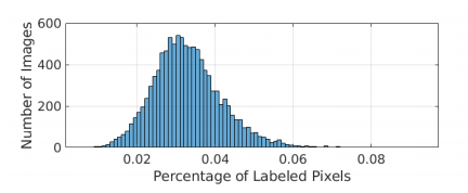
Only around 3% of pixels are labeled as 1 or 2 in the scribble annotation.

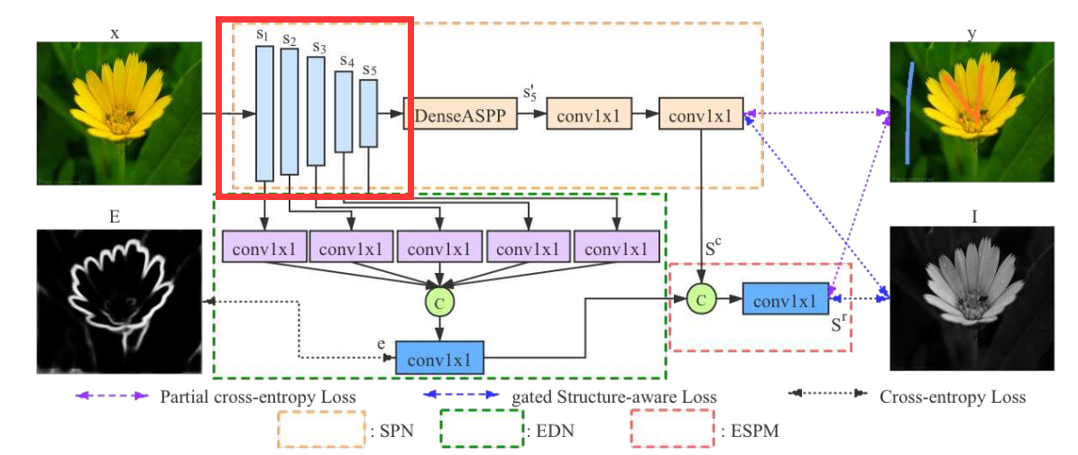
The structure of the network is shown below.

There are basically 3 main components in the network:

1. Saliency Prediction Network
2. Edge Detection Network
3. Edge-Enhanced Saliency Prediction Module

Weakly-Supervised SOD

Saliency Prediction Network (SPN)

Based on VGG16-Net, the front-end SPN is built by removing layers after the 5th pooling layer.

The convolutional layers that generate feature maps of the same resolution are grouped similar to:

Saining Xie and Zhuowen Tu. Holistically-nested edge detection. In Proc. IEEE Int. Conf. Comp. Vis., pages 1395–1403, 2015

Thus the front-end model is denoted as

\[f_1(x,\theta) = \{s_1,s_2,s_3,s_4,s_5\} \]

where \(s_i\) represents features from the last convolutional layer in the i-th stage stage, and \(\theta\) is its parameters.

The paper

Yunchao Wei, Huaxin Xiao, Honghui Shi, Zequn Jie, JiashiFeng, and Thomas S Huang. Revisiting dilated convolution: A simple approach for weakly- and semi- supervised semantic segmentation. In Proc. IEEE Conf. Comp. Vis. Patt.Recogn., pages 7268–7277, 2018.

suggests that larger fields by different dilation rates can spread the discriminative information to non-discriminative object regions.

A dense atrous spatial pyramid pooling module enlarges the receptive fields of feature \(s_5\).

Dense Atrous Spatial Pyramid Pooling（DASPP）_CSDN

In particular, different dilation rates are applied in the convolutional layers of DenseASPP.

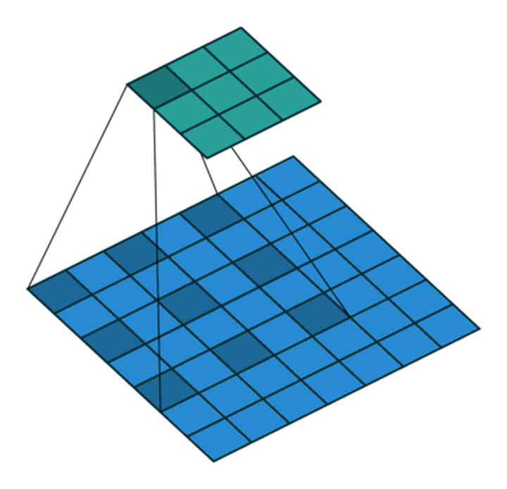
To enlarge receptive fields, there are 2 ways.

One way is to down-sample, but the side effect is it decreases the resolution.

The other way is to use Atrous Convolution, which can enlarge the receptive field while remaining the resolution.

Can we just iterate this process to achieve larger receptive fields?

Reason:

1. Prevent Gridding Effect

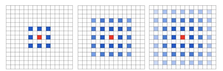
Not every pixel is used.

2. Balance large objects and small objects

Dilated Convolution with a 3 x 3 kernel and dilation rate 2

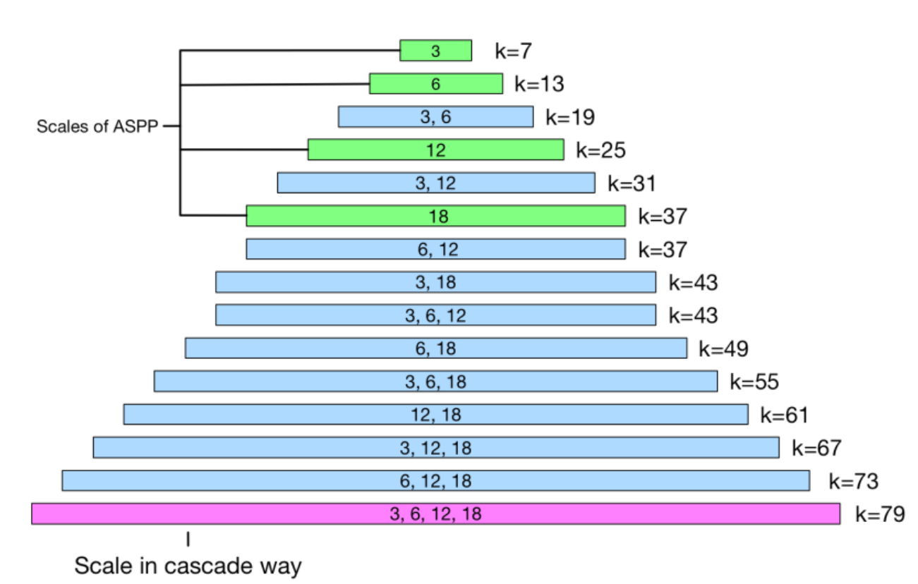
The numbers inside the rectangle denotes dilation rate, the length denotes kernel size, and k denotes actual receptive field size.

Then two \(1\times 1\) convolutional layers are used to map $s_5 ' $ into a one channel coarse saliency map \(s^c\).

To train the SPN, partial cross-entropy loss is adopted considering there are many unknown pixels.

\[\mathcal L_s = \sum _{(x,y) \in J_l} \mathcal L_{(x,y)} \]

where \(J_l\) represents the labeled pixel set.

Edge Detection Network (EDN)

EDN helps to produce saliency features with rich structure information.

Specifically, each \(s_i\) is mapped into a feature map of channel size \(M\) with a \(1\times 1\) convolutional layer

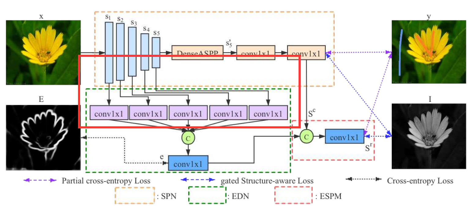
Then the 5 features maps are concatenated and fed to a \(1\times 1\) convolutional layer to produce an edge map \(e\).

A cross-entropy loss is used to train EDG

\[\mathcal L _e = \sum(E\log e + (1-E)\log(1-e)) \]

Where E is pre-computed by edge detector from the following paper.

Yun Liu, Ming-Ming Cheng, Xiaowei Hu, Kai Wang, and Xiang Bai. Richer convolutional features for edge detection. In Proc. IEEE Conf. Comp. Vis. Patt. Recogn., pages 3000–3009, 2017.

Edge-Enhanced Saliency Prediction Model (ESPM)

This model aims to refine the coarse saliency map \(s^c\) from SPN and obtain an edge-preserving refined saliency \(s^r\).

Specifically, \(s^c\) and \(e\) are concatenated and fed to a \(1\times 1\) convolutional layer.

Then we get \(s^r\) as the final output.

Similarly a partial cross-entropy loss is used to train ESPM.

\[\mathcal L_{s^r} = \sum _{(x,y) \in J_l} \mathcal L_{(x,y)} \]

Gated Structure-Aware Loss

It encourages the structure of a predicted saliency map to be similar to the salient region of the input image.

We want the predicted saliency map has consistent intensity in the salient region, and has a clear boundary.

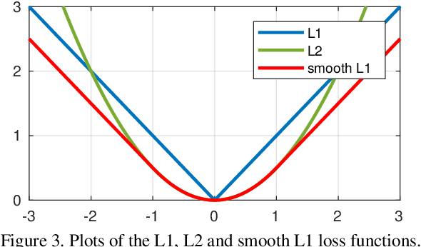
When x is small, it is more smooth than \(\mathrm L_1\) .

When x is big, its gradient is constant so it won't produce outrageous results due to outlier points.

This loss function can enforce smoothness while preserving structures.

However, SOD intends to suppress the structure information outside the salient regions.

Thus the smooth loss will make the predicted saliency map ambiguous.

To eliminate this ambiguity, a gated structure-aware loss is proposed to avoid the distraction from background structure.

\[\mathcal L _b = \sum_{(u,v)}\sum_{d\in (\bf x,\bf y)} \Psi (|\partial_d s_{(u,v)}|\exp (-\alpha |\partial _d(G\cdot I_{(u,v)})|)) \]

where \(\Psi(s) = \sqrt{s^2 + 1e^{-6}}\) , \(1e^{-6}\) is to avoid zero.

\(I_{(u,v)}\) denotes the image intensity at (u,v), \(d\) is the partial derivatives on the \(\bf x\) and \(\bf y\) directions.

\(G\) is the gate for the structure-aware loss. It applies \(\mathrm L_1\) penalty on gradients of \(s\) to encourage it to be locally smooth.

\(\partial I\) is used as weight to maintain saliency distinction along image edges.

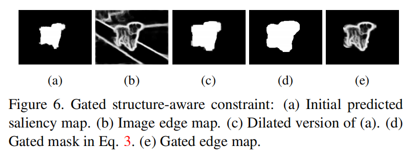
It can be seen that the network focus on saliency region and produce sharp boundaries.

Objective Function

Sum up previous loss functions we have

\[\mathcal L = \mathcal{L}_s(s^c,y) + \mathcal{L}_s(s^r,y) + \beta_1\mathcal{L}_b(s^c,x)+\beta_2\mathcal{L}_b(s^r,x) +\beta_3\mathcal{L}_e \]

The hyper-parameters are set as \(\alpha = 10\), \(\beta_1=\beta_2=0.3\), \(\beta_3=1\)

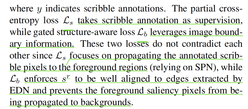
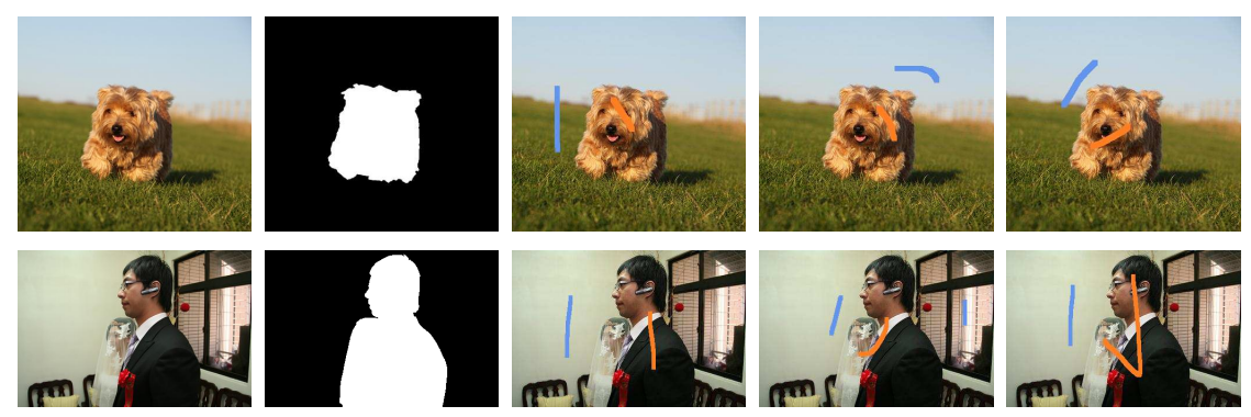
Scribble Boosting

Scribbles only annotate a very small part of the image.

This leads to local minima when it comes to complex shapes of objects.

(As is shown in (d) )

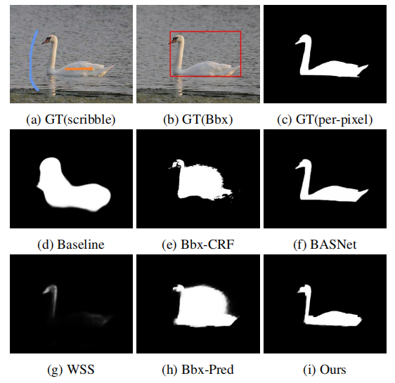
One simple way to deal with this problem is to use DenseCRF to expand scribble labels.

(e) is only slightly better than (d).

This is because the annotations are sparse and DenseCRF fails to make it denser.

So instead of directly expanding the scribbles, the DenseCRF is applied to the initial saliency prediction.

Then only the pixels with same value in both initial prediction and DenseCRF prediction are remained, as the DenseCRF prediction contains too much noise.

Others are labeled as unknown.

That's how new scribbles are obtained. (As is shown in (g), only one iteration )

Is more iterations better?

Then we feed the new scribbles into the network and obtain final results.

Saliency Structure Measure

Traditional evaluation metrics only focus on accuracy while neglecting how well the result complies with human perception.

In other words, good results should align with the structure of the object. (Sharp or ambigous)

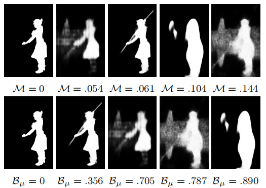
Thus BIOU loss \(B_\mu\) is adapted to evaluate the structure alignment.

\[B_\mu = 1 - \dfrac{2\sum(g_sg_y)}{\sum(g_s^2+g_y^2)} \]

where \(B_\mu \in [0,1]\).

The smaller \(B_\mu\) is , the better the results are.

To avoid unstable measurements due to the small scales of the edges, the edges are dilated with a \(3\times 3\) kernel first.

Experiments

S-DUTS dataset

An existing saliency dataset is relabeled with scribbles by 3 annotators.

Labeling with scribbles is easy and fast, which only takes 1~2 seconds on average.

Setup

The new network is trained on S-DUTS.

Then it's evaluated on 6 widely-used benchmarks.

DUTS, ECSSD, DUT, PASCAL-S, HKU-IS, THUR

There are 5 SOTA weakly-supervised/ unsupervised and 11 fully-supervised saliency object detection methods to be compared with.

Four evaluation metrics are used, including \(\mathrm {MAE}\), \(F_\beta\), \(E_\xi\) and newly proposed \(B_\mu\)

Comparison

Traditional weakly-supervised or unsupervised methods fail to capture structure information, leading to higher \(B_\mu\).

The new method achieves lower \(B_\mu\), and it's even comparable to some fully-supervised SOD methods.

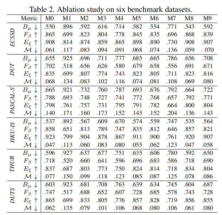
Ablation Study

graph NULL(("NULL")) --"Partial Cross-Entropy Loss"--> M1 M1--"Gated Structure-Aware Loss"--> M2 M1--"Smoothness Loss"-->M3 M1--"Edge Detection Network"-->M4 M2--"Edge Detection Network"-->M5 M4--"Gated Structure-Aware Loss"-->M5 M5--"DenseCRF Refinement"-->M6 M1--"Enlarge Annotation"--> M7 M5--"One Iteration"-->M0 M0--"Another Dataset"-->M8 M0--"Different Edge Detection Method"-->M9