机器学习 | 算法笔记- 逻辑斯蒂回归(Logistic Regression)
前言
本系列为机器学习算法的总结和归纳,目的为了清晰阐述算法原理,同时附带上手代码实例,便于理解。
目录
组合算法(Ensemble Method)
机器学习算法总结
本章为逻辑斯蒂回归,内容包括模型介绍及代码实现(包括自主实现和sklearn案例)。
一、算法简介
1.1 定义
逻辑斯蒂回归(Logistic Regression) 虽然名字中有回归,但模型最初是为了解决二分类问题。
线性回归模型帮助我们用最简单的线性方程实现了对数据的拟合,但只实现了回归而无法进行分类。因此LR就是在线性回归的基础上,构造的一种分类模型。
对线性模型进行分类如二分类任务,简单的是通过阶跃函数(unit-step function),即将线性模型的输出值套上一个函数进行分割,大于z的判定为0,小于z的判定为1。如下图左所示
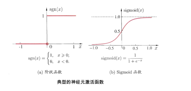
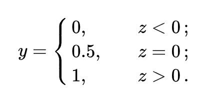
但这样的分段函数数学性质不好,既不连续也不可微。因此有人提出了对数几率函数,见上图右,简称Sigmoid函数。
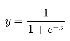
该函数具有很好的数学性质,既可以用于预测类别,并且任意阶可微,因此可用于求解最优解。将函数带进去,可得LR模型为
其实,LR 模型就是在拟合 z = w^T x +b 这条直线,使得这条直线尽可能地将原始数据中的两个类别正确的划分开。
1.2 损失函数
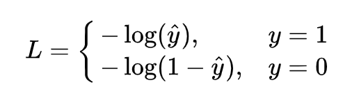
回归问题的损失函数一般为平均误差平方损失 MSE,LR解决二分类问题中,损失函数为如下形式
这个函数通常称为对数损失logloss,这里的对数底为自然对数 e ,其中真实值 y 是有 0/1 两种情况,而推测值 y^ 由于借助对数几率函数,其输出是介于0~1之间连续概率值。因此损失函数可以转换为分段函数
1.3 优化求解
确定损失函数后,要不断优化模型。LR的学习任务转化为数学的优化形式为
是一个关于w和b的函数。同样,采用梯度下降法进行求解,过程需要链式求导法则
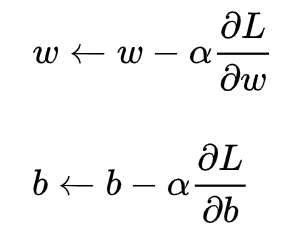
此处忽略求解过程。
此外,优化算法还包括
- Newton Method(牛顿法)
- Conjugate gradient method(共轭梯度法)
- Quasi-Newton Method(拟牛顿法)
- BFGS Method
- L-BFGS(Limited-memory BFGS)
上述优化算法中,BFGS与L-BFGS均由拟牛顿法引申出来,与梯度下降算法相比,其优点是:第一、不需要手动的选择步长;第二、比梯度下降算法快。但缺点是这些算法更加复杂,实用性不如梯度下降。
二、实例
2.1 自主实现
首先,建立 logistic_regression.py 文件,构建 LR 模型的类,内部实现了其核心的优化函数。


# -*- coding: utf-8 -*-

import numpy as np


class LogisticRegression(object):

    def __init__(self, learning_rate=0.1, max_iter=100, seed=None):
        self.seed = seed
        self.lr = learning_rate
        self.max_iter = max_iter

    def fit(self, x, y):
        np.random.seed(self.seed)
        self.w = np.random.normal(loc=0.0, scale=1.0, size=x.shape[1])
        self.b = np.random.normal(loc=0.0, scale=1.0)
        self.x = x
        self.y = y
        for i in range(self.max_iter):
            self._update_step()
            # print('loss: \t{}'.format(self.loss()))
            # print('score: \t{}'.format(self.score()))
            # print('w: \t{}'.format(self.w))
            # print('b: \t{}'.format(self.b))

    def _sigmoid(self, z):
        return 1.0 / (1.0 + np.exp(-z))

    def _f(self, x, w, b):
        z = x.dot(w) + b
        return self._sigmoid(z)

    def predict_proba(self, x=None):
        if x is None:
            x = self.x
        y_pred = self._f(x, self.w, self.b)
        return y_pred

    def predict(self, x=None):
        if x is None:
            x = self.x
        y_pred_proba = self._f(x, self.w, self.b)
        y_pred = np.array([0 if y_pred_proba[i] < 0.5 else 1 for i in range(len(y_pred_proba))])
        return y_pred

    def score(self, y_true=None, y_pred=None):
        if y_true is None or y_pred is None:
            y_true = self.y
            y_pred = self.predict()
        acc = np.mean([1 if y_true[i] == y_pred[i] else 0 for i in range(len(y_true))])
        return acc

    def loss(self, y_true=None, y_pred_proba=None):
        if y_true is None or y_pred_proba is None:
            y_true = self.y
            y_pred_proba = self.predict_proba()
        return np.mean(-1.0 * (y_true * np.log(y_pred_proba) + (1.0 - y_true) * np.log(1.0 - y_pred_proba)))

    def _calc_gradient(self):
        y_pred = self.predict()
        d_w = (y_pred - self.y).dot(self.x) / len(self.y)
        d_b = np.mean(y_pred - self.y)
        return d_w, d_b

    def _update_step(self):
        d_w, d_b = self._calc_gradient()
        self.w = self.w - self.lr * d_w
        self.b = self.b - self.lr * d_b
        return self.w, self.b
然后,这里我们创建了一个data_helper.py文件,单独用于创建模拟数据,并且内部实现了训练/测试数据的划分功能。
# -*- coding: utf-8 -*-

import numpy as np


def generate_data(seed):
    np.random.seed(seed)
    data_size_1 = 300
    x1_1 = np.random.normal(loc=5.0, scale=1.0, size=data_size_1)
    x2_1 = np.random.normal(loc=4.0, scale=1.0, size=data_size_1)
    y_1 = [0 for _ in range(data_size_1)]
    data_size_2 = 400
    x1_2 = np.random.normal(loc=10.0, scale=2.0, size=data_size_2)
    x2_2 = np.random.normal(loc=8.0, scale=2.0, size=data_size_2)
    y_2 = [1 for _ in range(data_size_2)]
    x1 = np.concatenate((x1_1, x1_2), axis=0)
    x2 = np.concatenate((x2_1, x2_2), axis=0)
    x = np.hstack((x1.reshape(-1,1), x2.reshape(-1,1)))
    y = np.concatenate((y_1, y_2), axis=0)
    data_size_all = data_size_1+data_size_2
    shuffled_index = np.random.permutation(data_size_all)
    x = x[shuffled_index]
    y = y[shuffled_index]
    return x, y

def train_test_split(x, y):
    split_index = int(len(y)*0.7)
    x_train = x[:split_index]
    y_train = y[:split_index]
    x_test = x[split_index:]
    y_test = y[split_index:]
    return x_train, y_train, x_test, y_test
最后,创建 train.py 文件,调用之前自己写的 LR 类模型实现分类任务,查看分类的精度。
# -*- coding: utf-8 -*-

import numpy as np
import matplotlib.pyplot as plt
import data_helper
from logistic_regression import *


# data generation
x, y = data_helper.generate_data(seed=272)
x_train, y_train, x_test, y_test = data_helper.train_test_split(x, y)

# visualize data
# plt.scatter(x_train[:,0], x_train[:,1], c=y_train, marker='.')
# plt.show()
# plt.scatter(x_test[:,0], x_test[:,1], c=y_test, marker='.')
# plt.show()

# data normalization
x_train = (x_train - np.min(x_train, axis=0)) / (np.max(x_train, axis=0) - np.min(x_train, axis=0))
x_test = (x_test - np.min(x_test, axis=0)) / (np.max(x_test, axis=0) - np.min(x_test, axis=0))

# Logistic regression classifier
clf = LogisticRegression(learning_rate=0.1, max_iter=500, seed=272)
clf.fit(x_train, y_train)

# plot the result
split_boundary_func = lambda x: (-clf.b - clf.w[0] * x) / clf.w[1]
xx = np.arange(0.1, 0.6, 0.1)
plt.scatter(x_train[:,0], x_train[:,1], c=y_train, marker='.')
plt.plot(xx, split_boundary_func(xx), c='red')
plt.show()

# loss on test set
y_test_pred = clf.predict(x_test)
y_test_pred_proba = clf.predict_proba(x_test)
print(clf.score(y_test, y_test_pred))
print(clf.loss(y_test, y_test_pred_proba))
# print(y_test_pred_proba)
2.2 sklearn
sklearn.linear_model模块提供了很多模型供我们使用,比如Logistic回归、Lasso回归、贝叶斯脊回归等,可见需要学习的东西还有很多很多。本篇文章,我们使用LogisticRegressioin。
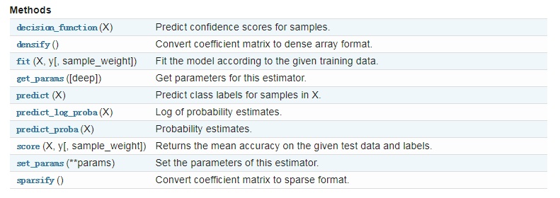
LogisticRegression这个函数,一共有14个参数,详见https://scikit-learn.org/dev/modules/generated/sklearn.linear_model.LogisticRegression.html
除此之外,LogisticRegression也有一些方法供我们使用:![]()
# -*- coding:UTF-8 -*-
from sklearn.linear_model import LogisticRegression

"""
函数说明:使用Sklearn构建Logistic回归分类器

Parameters:
    无
Returns:
    无

"""
def colicSklearn():
    frTrain = open('horseColicTraining.txt')                                        #打开训练集
    frTest = open('horseColicTest.txt')                                                #打开测试集
    trainingSet = []; trainingLabels = []
    testSet = []; testLabels = []
    for line in frTrain.readlines():
        currLine = line.strip().split('\t')
        lineArr = []
        for i in range(len(currLine)-1):
            lineArr.append(float(currLine[i]))
        trainingSet.append(lineArr)
        trainingLabels.append(float(currLine[-1]))
    for line in frTest.readlines():
        currLine = line.strip().split('\t')
        lineArr =[]
        for i in range(len(currLine)-1):
            lineArr.append(float(currLine[i]))
        testSet.append(lineArr)
        testLabels.append(float(currLine[-1]))
    classifier = LogisticRegression(solver='liblinear',max_iter=10).fit(trainingSet, trainingLabels)
    test_accurcy = classifier.score(testSet, testLabels) * 100
    print('正确率:%f%%' % test_accurcy)

if __name__ == '__main__':
    colicSklearn()

 浙公网安备 33010602011771号