自动求导(Automatic Derivatives)
现在考虑自动微分;
下面代码片段实现了Rat43自动微分的代价函数
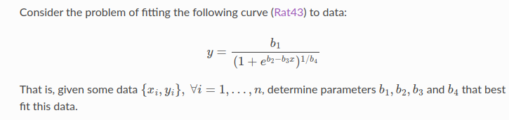
上面可以表述为:找到b1,b2,b3,b4的值来最小化下面的目标函数
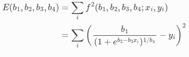
使用Ceres Solver来解决这个问题,我们需要定义一个代价函数(CostFunction)在给定的x和y上计算残差f以及该残差相对于b1,b2,b3,b4的导数。
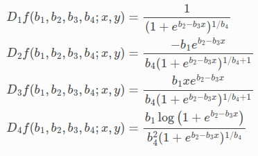
对b1,b2,b3,b4求导如下:
有了这些导数,可以实现代价函数(CostFunction):
class Rat43Analytic : public SizedCostFunction<1,4> {
   public:
     Rat43Analytic(const double x, const double y) : x_(x), y_(y) {}
     virtual ~Rat43Analytic() {}
     virtual bool Evaluate(double const* const* parameters,
                           double* residuals,
                           double** jacobians) const {
       const double b1 = parameters[0][0];
       const double b2 = parameters[0][1];
       const double b3 = parameters[0][2];
       const double b4 = parameters[0][3];

       residuals[0] = b1 *  pow(1 + exp(b2 -  b3 * x_), -1.0 / b4) - y_;

       if (!jacobians) return true;
       double* jacobian = jacobians[0];
       if (!jacobian) return true;

       jacobian[0] = pow(1 + exp(b2 - b3 * x_), -1.0 / b4);
       jacobian[1] = -b1 * exp(b2 - b3 * x_) *
                     pow(1 + exp(b2 - b3 * x_), -1.0 / b4 - 1) / b4;
       jacobian[2] = x_ * b1 * exp(b2 - b3 * x_) *
                     pow(1 + exp(b2 - b3 * x_), -1.0 / b4 - 1) / b4;
       jacobian[3] = b1 * log(1 + exp(b2 - b3 * x_)) *
                     pow(1 + exp(b2 - b3 * x_), -1.0 / b4) / (b4 * b4);
       return true;
     }

    private:
     const double x_;
     const double y_;
 };
在实际实现中,不适用上面的方式,因为会相对很耗时:
实际中实现如下:
class Rat43AnalyticOptimized : public SizedCostFunction<1,4> {
   public:
     Rat43AnalyticOptimized(const double x, const double y) : x_(x), y_(y) {}
     virtual ~Rat43AnalyticOptimized() {}
     virtual bool Evaluate(double const* const* parameters,
                           double* residuals,
                           double** jacobians) const {
       const double b1 = parameters[0][0];
       const double b2 = parameters[0][1];
       const double b3 = parameters[0][2];
       const double b4 = parameters[0][3];

       const double t1 = exp(b2 -  b3 * x_);
       const double t2 = 1 + t1;
       const double t3 = pow(t2, -1.0 / b4);
       residuals[0] = b1 * t3 - y_;

       if (!jacobians) return true;
       double* jacobian = jacobians[0];
       if (!jacobian) return true;

       const double t4 = pow(t2, -1.0 / b4 - 1);
       jacobian[0] = t3;
       jacobian[1] = -b1 * t1 * t4 / b4;
       jacobian[2] = -x_ * jacobian[1];
       jacobian[3] = b1 * log(t2) * t3 / (b4 * b4);
       return true;
     }

   private:
     const double x_;
     const double y_;
 };
上面是解析求导,为了引出Rat43,顺便就把解析求导也给出了。
下面正式分析自动求导:
自动求导的代码如下:
struct Rat43CostFunctor {
  Rat43CostFunctor(const double x, const double y) : x_(x), y_(y) {}

  template <typename T>
  bool operator()(const T* parameters, T* residuals) const {
    const T b1 = parameters[0];
    const T b2 = parameters[1];
    const T b3 = parameters[2];
    const T b4 = parameters[3];
    residuals[0] = b1 * pow(1.0 + exp(b2 -  b3 * x_), -1.0 / b4) - y_;
    return true;
  }

  private:
    const double x_;
    const double y_;
};


CostFunction* cost_function =
      new AutoDiffCostFunction<Rat43CostFunctor, 1, 4>(//残差维数,变量维数
        new Rat43CostFunctor(x, y));
为了知道自动求导怎么工作的,需要先学习一下Dual Numbers以及Jets
Dual Numbers和Jets
注意:对于使用ceres solver中的自动求导,阅读这部分以及下部分关于实现Jets不是必须的。但是知道Jets是怎样工作的基本知识是有必要的,尤其是当调试和推导自动求导的性能的时候。
Dual 数字是实数的扩展类似于复数;然而复数增加了实数通过引入单位虚数l2 = -1,dual 数字引入了一个无穷小单位e,它的平方为0.一个dual 数字a + ve有两个部分,实部a和无穷小部v。
神奇的是,这个简单的改变导致一个方便的方法用于精确计算导数而不需要操作复杂的负号表达式。
例如:
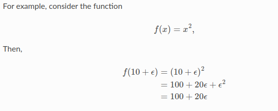
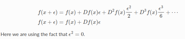
可以观察e的系数是Df(10) = 20.事实上,这推广到非多项式函数。考虑一个任意可微函数f(x).然后我们可以通过考虑在x附近的泰勒展开来评价f(x+e),给出一个无穷级数:
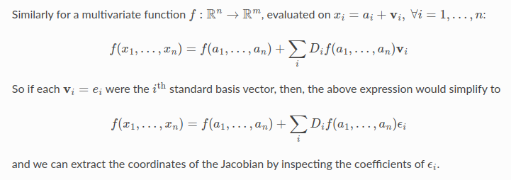
一个Jet是一个n维的dual 数字,我们用n维的无穷小ei,来扩展实数,i=1,...,n,对于任意i,j,eiej=0.那一个Jet由一个实部a和一个n维的无穷小v组成,如

上面求和负号比较冗长,给出简介的写法:

上面ei是隐含了的。然后,运用同样的泰勒展开,可以得出:

以此类推,
实现Jets
对于以上在实践工作中,我们需要评价任意函数f不仅在实数上还是在dual数上的能力,dual数通常不是评价他们的泰勒展开来评价函数。
这就是C++模板和运算符重载发挥作用的地方,以下代码片段是对Jet的简单的实现,包括一些对他们操作的函数和操作符。
template<int N> struct Jet{
 double a;
 Eigen::Matrix<double, 1, N> v;
};

template<int N> Jet<N> operator+(const Jet<N>& f, const Jet<N>& g)
{
return Jet<N>(f.a + g.a, f.v +g.v);
}
template<int N> Jet<N> operator-(const Jet<N>& f, const Jet<N>& g) {
  return Jet<N>(f.a - g.a, f.v - g.v);
}
template<int N> Jet<N> operator*(const Jet<N>& f, const Jet<N>& g) {
  return Jet<N>(f.a * g.a, f.a * g.v + f.v * g.a);
}

template<int N> Jet<N> operator/(const Jet<N>& f, const Jet<N>& g) {
  return Jet<N>(f.a / g.a, f.v / g.a - f.a * g.v / (g.a * g.a));
}
template <int N> Jet<N> exp(const Jet<N>& f) {
  return Jet<T, N>(exp(f.a), exp(f.a) * f.v);
}

// This is a simple implementation for illustration purposes, the
// actual implementation of pow requires careful handling of a number
// of corner cases.
template <int N>  Jet<N> pow(const Jet<N>& f, const Jet<N>& g) {
  return Jet<N>(pow(f.a, g.a),
                g.a * pow(f.a, g.a - 1.0) * f.v +
                pow(f.a, g.a) * log(f.a); * g.v);
}
有了这些重载的函数,我们可以调用Rat43CostFunctor带有Jets的数组而不是浮点数。将合适的初始Jets组合起来以便计算雅克比如下:
class Rat43Automatic : public ceres::SizedCostFunction<1,4> {
 public:
  Rat43Automatic(const Rat43CostFunctor* functor) : functor_(functor) {}
  virtual ~Rat43Automatic() {}
  virtual bool Evaluate(double const* const* parameters,
                        double* residuals,
                        double** jacobians) const {
    // Just evaluate the residuals if Jacobians are not required.
    if (!jacobians) return (*functor_)(parameters[0], residuals);

    // Initialize the Jets
    ceres::Jet<4> jets[4];
    for (int i = 0; i < 4; ++i) {
      jets[i].a = parameters[0][i];
      jets[i].v.setZero();
      jets[i].v[i] = 1.0;
    }

    ceres::Jet<4> result;
    (*functor_)(jets, &result);

    // Copy the values out of the Jet.
    residuals[0] = result.a;
    for (int i = 0; i < 4; ++i) {
      jacobians[0][i] = result.v[i];
    }
    return true;
  }

 private:
  std::unique_ptr<const Rat43CostFunctor> functor_;
};
这就是AutoDiffCostFunction工作的实质;
可以看出Jet的实部为残差,虚部为雅克比;
一些困难
自动求导让用户免于求雅克比的麻烦,但是有代价的,例如,考虑以下的简单functor:
struct Functor {
  template <typename T> bool operator()(const T* x, T* residual) const {
    residual[0] = 1.0 - sqrt(x[0] * x[0] + x[1] * x[1]);
    return true;
  }
};
上面是残差的计算,没有预见性的问题;但是如果对于雅克比的解析表达式,如下
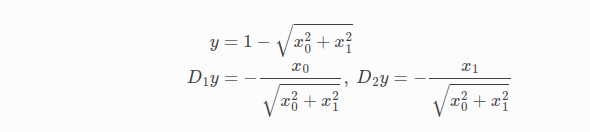
可以看出,当x0=x1=0时,这是一个不确定的形式。
这个问题没有单一的解决方法。
Interfacing with Automatic Differentiation
在代价函数的显示表达式可用的情况下,自动求导是直截了当的。但是这并不总是可能的。通常必须与外部例程或数据交互。本章给出了一些方法。
考虑找到theta和t来优化下面形式的问题:

R是一个二维的旋转矩阵用theta来参数化,t是一个二维的向量,f是一个外部的畸变函数。
有一个模板函数TemplatedComputeDistortion可以计算f,对应的残差functor的实现是直截了当的
template <typename T> T TemplatedComputeDistortion(const T r2) {
  const double k1 = 0.0082;
  const double k2 = 0.000023;
  return 1.0 + k1 * r2 + k2 * r2 * r2;
}

struct Affine2DWithDistortion {
  Affine2DWithDistortion(const double x_in[2], const double y_in[2]) {
    x[0] = x_in[0];
    x[1] = x_in[1];
    y[0] = y_in[0];
    y[1] = y_in[1];
  }

  template <typename T>
  bool operator()(const T* theta,
                  const T* t,
                  T* residuals) const {
    const T q_0 =  cos(theta[0]) * x[0] - sin(theta[0]) * x[1] + t[0];
    const T q_1 =  sin(theta[0]) * x[0] + cos(theta[0]) * x[1] + t[1];
    const T f = TemplatedComputeDistortion(q_0 * q_0 + q_1 * q_1);
    residuals[0] = y[0] - f * q_0;
    residuals[1] = y[1] - f * q_1;
    return true;
  }

  double x[2];
  double y[2];
};
目前还好,但是考虑三种方法定义f,其不直接适用于自动微分:
1.计算其值的非模板函数;
2.计算其值和导数的函数;
3.定义为要插值的值表的函数;
返回它的值的函数(A function that returns its value)
假设给定一个函数ComputeDistortionValue,如下
double ComputeDistortionValue(double r2);
它计算了f的值。函数实际的实现不重要。与函数Affine2DWithDistortion交互需要三个步骤:
1.Wrap ComputeDistortionValue into a functor ComputeDistortionValueFunctor.
struct ComputeDistortionValueFunctor {
  bool operator()(const double* r2, double* value) const {
    *value = ComputeDistortionValue(r2[0]);
    return true;
  }
};
2.Numerically differentiate ComputeDistortionValueFunctor using NumericDiffCostFunction to create a CostFunction.
3.Wrap the resulting CostFunction object using CostFunctionToFunctor. The resulting object is a functor with a templated operator() method, which pipes the Jacobian computed by NumericDiffCostFunction into the appropriate Jet objects.
具体实现如下:
struct ComputeDistortionValueFunctor {
  bool operator()(const double* r2, double* value) const {
    *value = ComputeDistortionValue(r2[0]);
    return true;
  }
};

struct Affine2DWithDistortion {
  Affine2DWithDistortion(const double x_in[2], const double y_in[2]) {
    x[0] = x_in[0];
    x[1] = x_in[1];
    y[0] = y_in[0];
    y[1] = y_in[1];

    compute_distortion.reset(new ceres::CostFunctionToFunctor<1, 1>(
         new ceres::NumericDiffCostFunction<ComputeDistortionValueFunctor,
                                            ceres::CENTRAL,
                                            1,
                                            1>(
            new ComputeDistortionValueFunctor)));
  }

  template <typename T>
  bool operator()(const T* theta, const T* t, T* residuals) const {
    const T q_0 = cos(theta[0]) * x[0] - sin(theta[0]) * x[1] + t[0];
    const T q_1 = sin(theta[0]) * x[0] + cos(theta[0]) * x[1] + t[1];
    const T r2 = q_0 * q_0 + q_1 * q_1;
    T f;
    (*compute_distortion)(&r2, &f);
    residuals[0] = y[0] - f * q_0;
    residuals[1] = y[1] - f * q_1;
    return true;
  }

  double x[2];
  double y[2];
  std::unique_ptr<ceres::CostFunctionToFunctor<1, 1> > compute_distortion;
};
函数返回它的值和导数(A function that returns its value and derivative)
假设给定一个函数ComputeDistortionValue,它能够计算其值和可选的雅克比,有以下形式:
void ComputeDistortionValueAndJacobian(double r2,
                                       double* value,
                                       double* jacobian);
同样的这个函数具体的实现不重要。用Affine2DWithDistortion函数与上面函数对接,有两步:
1.Wrap ComputeDistortionValueAndJacobian into a CostFunction object which we call ComputeDistortionFunction.
class ComputeDistortionFunction : public ceres::SizedCostFunction<1, 1> {
 public:
  virtual bool Evaluate(double const* const* parameters,
                        double* residuals,
                        double** jacobians) const {
    if (!jacobians) {
      ComputeDistortionValueAndJacobian(parameters[0][0], residuals, nullptr);
    } else {
      ComputeDistortionValueAndJacobian(parameters[0][0], residuals, jacobians[0]);
    }
    return true;
  }
};

struct Affine2DWithDistortion {
  Affine2DWithDistortion(const double x_in[2], const double y_in[2]) {
    x[0] = x_in[0];
    x[1] = x_in[1];
    y[0] = y_in[0];
    y[1] = y_in[1];
    compute_distortion.reset(
        new ceres::CostFunctionToFunctor<1, 1>(new ComputeDistortionFunction));
  }

  template <typename T>
  bool operator()(const T* theta,
                  const T* t,
                  T* residuals) const {
    const T q_0 =  cos(theta[0]) * x[0] - sin(theta[0]) * x[1] + t[0];
    const T q_1 =  sin(theta[0]) * x[0] + cos(theta[0]) * x[1] + t[1];
    const T r2 = q_0 * q_0 + q_1 * q_1;
    T f;
    (*compute_distortion)(&r2, &f);
    residuals[0] = y[0] - f * q_0;
    residuals[1] = y[1] - f * q_1;
    return true;
  }

  double x[2];
  double y[2];
  std::unique_ptr<ceres::CostFunctionToFunctor<1, 1> > compute_distortion;
};
后面的不是很明白!


 浙公网安备 33010602011771号