单变量线性回归模型

1.模型描述

拟合函数
\(h_{\theta}(x)=\theta_{0}+\theta_{1} x\)
\(x=(x^{(1)},x^{(2)}...x^{(m)})\)训练集
\(h=(h^{(1)},h^{(2)}...h^{(m)})\)训练集
共m个样本

参数

\(\theta_{0}\)是回归系数
\(\theta_{1}\)是常数项,均是未知的
在线性模型中，就是找到一个样本\((x^(i),y^(i))\)得到最近接真实值的参数\(a\)和\(b\),进而得到线性模型

代价函数/损失函数

参考知乎
预测值与实际值差的平方和的最小值
取值才能让这条直线最佳地拟合这些数据呢？这就是代价函数登场的时刻了
\(J\left(\theta_{0}, \theta_{1}\right)=\frac{1}{2 m} \sum_{i=1}^{m}\left(\hat{y}_{i}-y_{i}\right)^{2}=\frac{1}{2 m} \sum_{i=1}^{m}\left(h_{\theta}\left(x_{i}\right)-y_{i}\right)^{2}\)

这就是一次函数的代价函数 \(J\left(\theta_{0}, \theta_{1}\right)\)。

判断拟合的这个函数是否准确就是判断通过这个函数的出来的结果与实际结果有多大的误差：

\(\left(h_{\theta}\left(x_{i}\right)-y_{i}\right)^{2}\)

i 为第 i 个数据，上式表示我通过拟合函数 \(h_{\theta}(x)\)得到的第 i 个数据与真实的第 i 个数据的误差。总共有 m 个数据，那么我们就应该把 m 个数据的误差求和然后再求出平均误差，得到下面这个式子。

\(\frac{1}{2 m} \sum_{i=1}^{m}\left(h_{\theta}\left(x_{i}\right)-y_{i}\right)^{2}\)
只要我让这个值尽可能的小，我所做的拟合函数就越准确，那么刚才求拟合函数的问题就转化成了通过 \(θ_0\) 和 \(θ_1\)求\(J\left(\theta_{0}, \theta_{1}\right)\)的最小值。
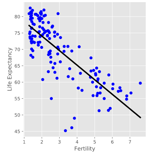
给出一个gaminder数据集上面的单变量回归模型
直接使用sklearn包里面的线性回归即可

# Import LinearRegression
from sklearn.linear_model import LinearRegression

# Create the regressor: reg
reg = LinearRegression()

# Create the prediction space
prediction_space = np.linspace(min(X_fertility), max(X_fertility)).reshape(-1,1)

# Fit the model to the data
reg.fit(X_fertility, y)

# Compute predictions over the prediction space: y_pred
y_pred = reg.predict(prediction_space)

# Print R^2 
print(reg.score(X_fertility, y))

# Plot regression line
plt.plot(prediction_space, y_pred, color='black', linewidth=3)
plt.show()
#因为是一个基本模型，因此误差很大
<script.py> output:
    0.6192442167740035

# Import necessary modules
from sklearn.linear_model import LinearRegression
from sklearn.metrics import mean_squared_error
from sklearn.model_selection import train_test_split

# Create training and test sets
X_train, X_test, y_train, y_test = train_test_split(X, y, test_size = 0.3, random_state=42)

# Create the regressor: reg_all
reg_all = LinearRegression()

# Fit the regressor to the training data
reg_all.fit(X_train, y_train)

# Predict on the test data: y_pred
y_pred = reg_all.predict(X_test)

# Compute and print R^2 and RMSE
print("R^2: {}".format(reg_all.score(X_test, y_test)))
rmse = np.sqrt(mean_squared_error(y_test, y_pred))
print("Root Mean Squared Error: {}".format(rmse))

<script.py> output:
    R^2: 0.838046873142936
    Root Mean Squared Error: 3.2476010800377213

如果有人比较懒，不希望每次都要亲自处理这些数据，从代价函数图中找到最小值所在的点。有没有一种算法可以自动地求出使得代价函数最小的点呢？有，那就是梯度下降