RBF网络的matlab实现

一、用工具箱实现函数拟合

参考：http://blog.csdn.net/zb1165048017/article/details/49407075

(1)newrb()

该函数可以用来设计一个近似径向基网络(approximate RBF)。调用格式为：

[net,tr]=newrb(P,T,GOAL,SPREAD,MN,DF)

其中P为Q组输入向量组成的R*Q位矩阵，T为Q组目标分类向量组成的S*Q维矩阵。GOAL为均方误差目标(Mean Squard Error Goal)，默认为0.0；SPREAD为径向基函数的扩展速度，默认为1；MN为神经元的最大数目，默认为Q；DF维两次显示之间所添加的神经元数目，默认为25；ner为返回值，一个RBF网络，tr为返回值，训练记录。

用newrb（）创建RBF网络是一个不断尝试的过程(从程序的运行可以看出来)，在创建过程中，需要不断增加中间层神经元的和个数，知道网络的输出误差满足预先设定的值为止。

(2)newrbe()

该函数用于设计一个精确径向基网络(exact RBF)，调用格式为：

net=newrbe(P,T,SPREAD)

其中P为Q组输入向量组成的R*Q维矩阵，T为Q组目标分类向量组成的S*Q维矩阵；SPREAD为径向基函数的扩展速度，默认为1

和newrb()不同的是，newrbe()能够基于设计向量快速，无误差地设计一个径向基网络。

(3)radbas()

该函数为径向基传递函数，调用格式为

A=radbas(N)

info=radbas(code)

其中N为输入（列）向量的S*Q维矩阵，A为函数返回矩阵，与N一一对应，即N的每个元素通过径向基函数得到A；info=radbas(code)表示根据code值的不同返回有关函数的不同信息。包括

derive——返回导函数的名称

name——返回函数全称

output——返回输入范围

active——返回可用输入范围

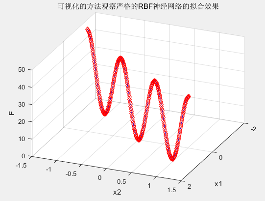
使用exact径向基网络来实现非线性的函数回归：

%%清空环境变量  
clc
clear
%%产生输入输出数据  
%设置步长  
interval=0.01;
%产生x1,x2  
x1=-1.5:interval:1.5;
x2=-1.5:interval:1.5;
%按照函数先求的响应的函数值，作为网络的输出  
F=20+x1.^2-10*cos(2*pi*x1)+x2.^2-10*cos(2*pi*x2);
%%网络建立和训练  
%网络建立，输入为[x1;x2]，输出为F。spread使用默认  
net=newrbe([x1;x2],F);
%%网络的效果验证  
%将原数据回带，测试网络效果  
ty=sim(net,[x1;x2]);
%%使用图像来看网络对非线性函数的拟合效果  
figure
plot3(x1,x2,F,'rd');
hold on;
plot3(x1,x2,ty,'b-.');
view(113,36);
title('可视化的方法观察严格的RBF神经网络的拟合效果');
xlabel('x1')
ylabel('x2')
zlabel('F')
grid on

　　结果：

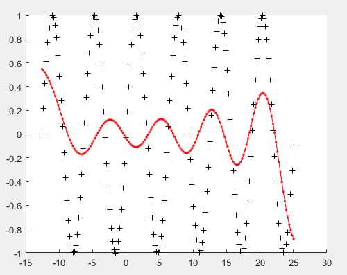
二、自编函数实现拟合

clear;
%X=1:100;
X=[-4*pi:0.07*pi:8*pi];  
P=length(X);
Y=[];
M=10; 
centers=[];
deltas=[]; 
weights=[];
set = {}; 
gap=0.1; 
%**************************************************************************  
%构造训练样本X,Y  
X=[-4*pi:0.07*pi:8*pi];  
for i=1:P  
    Y(i)=sin(X(i));
end 
%**************************************************************************  
for i=1:M                          %先随意初始化M个中心点
    centers(i)= X( i*floor( P/10 ) );  
end 
done=0;  
while(~done)  
    for i=1:M  
       set{i}=[];  
    end 
    for i=1:P  
        distance=100;
        for j=1:M  
            curr=abs(X(i)-centers(j));  
            if curr<distance  
                sets=j;  
                distance=curr;  
            end 
        end 
        set{sets}=[set{sets},X(i)];        %聚类，找出M个中心点，并且样本分布在这十个点周围
    end
    for i=1:M  
        new_centers(i)=sum(set{i})/length(set{i}); %重新计算中心点：M个类里每个类的中心点  
    end 
    done=0;  
     for i=1:M  
          sum1(i)=abs(centers(i)-new_centers(i));
     end 
     if sum(sum1)>gap  
            done=0;      %不断循环，直到找到最佳的中心点；
            centers=new_centers;  
     else 
            done=1;  
     end    
end
 
for i=1:M
    curr=abs( centers-centers(i));  
    [curr_2,b]=min(curr);  
    curr(b)=100;  
    curr_2=min(curr);  
    deltas(i)=1*curr_2;  
end
%{
for i=1:M
    sum=0;
    num=length(set{i});
    for j=1:num
        sum=sum+(set{i}(j)-centers(i))^2;
    end
    deltas(i)=(sum)^0.5/num;
end
%}
for i=1:P  
    for j=1:M  
        curr=abs(X(i)-centers(j));  
        K(i,j)=exp( -curr^2/(2*deltas(j)^2) );  %隐含层的输出
    end 
end 
%计算权值矩阵  
weights=inv(K'*K)*K'*Y';  
%**************************************************************************  
%测试计算出函数的情况  
x_test=[-4*pi:0.07*pi:8*pi];    
for i=1:length(x_test)  
    sum=0;  
    for j=1:M  
        curr=weights(j)*exp(-abs(x_test(i)-centers(j))^2/(2*deltas(j)^2));  
        sum=sum+curr;  
    end 
    y_test(i)=sum;  
end 
figure(1)  
scatter(X,Y,'k+');  
hold on;  
plot(x_test,y_test,'r.-')

结果：

三、工具箱函数的RBF分类

train_data=LowDimFaces(1:10,:);  %train_data是一个10*20维的矩阵，其中行表示样本数，列数表示特征个数
train_label=[ones(1,5),zeros(1,5)]; %行向量
 
display('读入测试数据...');
 
test_data=LowDimFaces(201:210,:);
test_label=[ones(1,5),zeros(1,5)];
 
[train_data,minX,maxX] = premnmx(train_data);
test_data = tramnmx(test_data,minX,maxX) ;
 
%网络建立，输入为[x1;x2]，输出为F。spread使用默认  
net=newrbe(train_data',train_label);
%%网络的效果验证  
%将原数据回带，测试网络效果  
ty=sim(net,test_data');
%%使用图像来看网络对非线性函数的拟合效果  
Y=[];
hitnum=0;
for i=1:10
    if ty(i)>0.5
        Y(i)=1;
    else
        Y(i)=0;
    end
    if Y(i)==test_label(i)
        hitnum=hitnum+1;
    end
end
fprintf('训练集中结果的正确率是%f%%\n',100*hitnum/10);

四、自编函数实现RBF分类

100

101

102

103

104

105

106

107

108

109

110

111

112

clear;
clc;
M=10; 
centers=[;];
deltas=[]; 
weights=[];
set = {}; 
gap=0.1; 
%**************************************************************************  
XA=ones(1,500);
YA=ones(1,500);  %初始化A类的输入数据
XB=ones(1,500);
YB=ones(1,500);  %初始化B类的输入数据
for i=1:500
    XA(i)=cos(2*pi*(i+8)/25-0.25*pi)*(i+8)/25;
    YA(i)=sin(2*pi*(i+8)/25-0.25*pi)*(i+8)/25-0.25;
    XB(i)=sin(2*pi*(i+8)/25+0.25*pi)*(i+8)/-25;
    YB(i)=cos(2*pi*(i+8)/25+0.25*pi)*(i+8)/25-0.25;
end
scatter(XA,YA,20,'b');
hold on;
scatter(XB,YB,20,'k');
hold off;
X1=cat(1,XA,YA);
X2=cat(1,XB,YB);
X=cat(2,X1,X2);  %得到训练数据集X,Y
Y=zeros(1,1000);
Y(1,1:500)=1;
k=rand(1,1000);
[m,n]=sort(k);
X=X(:,n(1:1000));
Y=Y(:,n(1:1000));
%**************************************************************************  
[X,minX,maxX] = premnmx(X);
P=length(X);
for i=1:M                          %先随意初始化M个中心点
    centers(:,i)= X(:,i*floor( P/10 ) );  
end 
done=0;  
while(~done)  
    for i=1:M  
       set{i}=[;];  
    end 
    for i=1:P  
        distance=100;
        for j=1:M  
            curr=norm(X(:,i)-centers(:,j));  
            if curr<distance  
                sets=j;  
                distance=curr;  
            end 
        end 
        set{sets}=[set{sets},X(:,i)];        %聚类，找出M个中心点，并且样本分布在这十个点周围
    end
    for i=1:M  
        new_centers(:,i)=sum(set{i}')'/length(set{i}); %重新计算中心点：M个类里每个类的中心点  
    end 
    done=0;  
     for i=1:M  
          sum1(i)=norm(centers(:,i)-new_centers(:,i));
     end 
     if sum(sum1)>gap  
            done=0;      %不断循环，直到找到最佳的中心点；
            centers=new_centers;  
     else 
            done=1;  
     end    
end
 
for i=1:M
    curr=[;];
    curr=abs( bsxfun(@minus,centers,centers(:,i)));
    k=100;
    m=norm(curr(:,j));
    for j=1:M
        if m<k && m~=0
            k=m;
        end
    end
    deltas(i)=k; 
end
 
 
for i=1:P  
    for j=1:M  
        curr=norm(X(:,i)-centers(:,j));  
        K(i,j)=exp( -curr^2/(2*deltas(j)^2) );  %隐含层的输出
    end 
end 
%计算权值矩阵  
weights=inv(K'*K)*K'*Y';  
%**************************************************************************  
%测试计算出函数的情况  
x_test=X;
for i=1:length(x_test)  
    sum=0;  
    for j=1:M  
        curr=weights(j)*exp(-norm(x_test(:,i)-centers(:,j))^2/(2*deltas(j)^2));  
        sum=sum+curr;  
    end 
    y_test(i)=sum;  
end
y_test(find(y_test<0.5))=0;
y_test(find(y_test>=0.5))=1;
count=0;
for j=1:length(y_test)
    if y_test(j)==Y(j)
        count=count+1;
    end
end
fprintf('分类正确率为：%.2f%%',100*count/length(y_test));
    