实验二：逻辑回归算法实验

|博客班级|https://edu.cnblogs.com/campus/czu/classof2020BigDataClass3-MachineLearning|

|----|----|----|

|作业要求|https://edu.cnblogs.com/campus/czu/classof2020BigDataClass3-MachineLearning/homework/12858|

|学号|201613324|

【实验目的】

理解逻辑回归算法原理，掌握逻辑回归算法框架；
理解逻辑回归的sigmoid函数；
理解逻辑回归的损失函数；
针对特定应用场景及数据，能应用逻辑回归算法解决实际分类问题。

【实验内容】

1.根据给定的数据集，编写python代码完成逻辑回归算法程序，实现如下功能：

建立一个逻辑回归模型来预测一个学生是否会被大学录取。假设您是大学部门的管理员，您想根据申请人的两次考试成绩来确定他们的入学机会。您有来自以前申请人的历史数据，可以用作逻辑回归的训练集。对于每个培训示例，都有申请人的两次考试成绩和录取决定。您的任务是建立一个分类模型，根据这两门考试的分数估计申请人被录取的概率。
算法步骤与要求：

(1)读取数据；(2)绘制数据观察数据分布情况；(3)编写sigmoid函数代码；(4)编写逻辑回归代价函数代码；(5)编写梯度函数代码；(6)编写寻找最优化参数代码（可使用scipy.opt.fmin_tnc()函数）；(7)编写模型评估（预测）代码，输出预测准确率；(8)寻找决策边界，画出决策边界直线图。

2. 针对iris数据集，应用sklearn库的逻辑回归算法进行类别预测。

要求：

（1）使用seaborn库进行数据可视化；（2）将iri数据集分为训练集和测试集(两者比例为8:2)进行三分类训练和预测；（3）输出分类结果的混淆矩阵。

【实验报告要求】

对照实验内容，撰写实验过程、算法及测试结果；
代码规范化：命名规则、注释；
实验报告中需要显示并说明涉及的数学原理公式；
查阅文献，讨论逻辑回归算法的应用场景；

实验内容及结果

问题一

1.读取数据

import numpy as np
import pandas as pd
import matplotlib.pyplot as plt
data=pd.read_csv("C:\\Users\\86152\\Desktop\\ex2data1.txt",delimiter=',',header=None,names=['exam1','exam2','isAdmitted'])
data.head(5)
print(data)

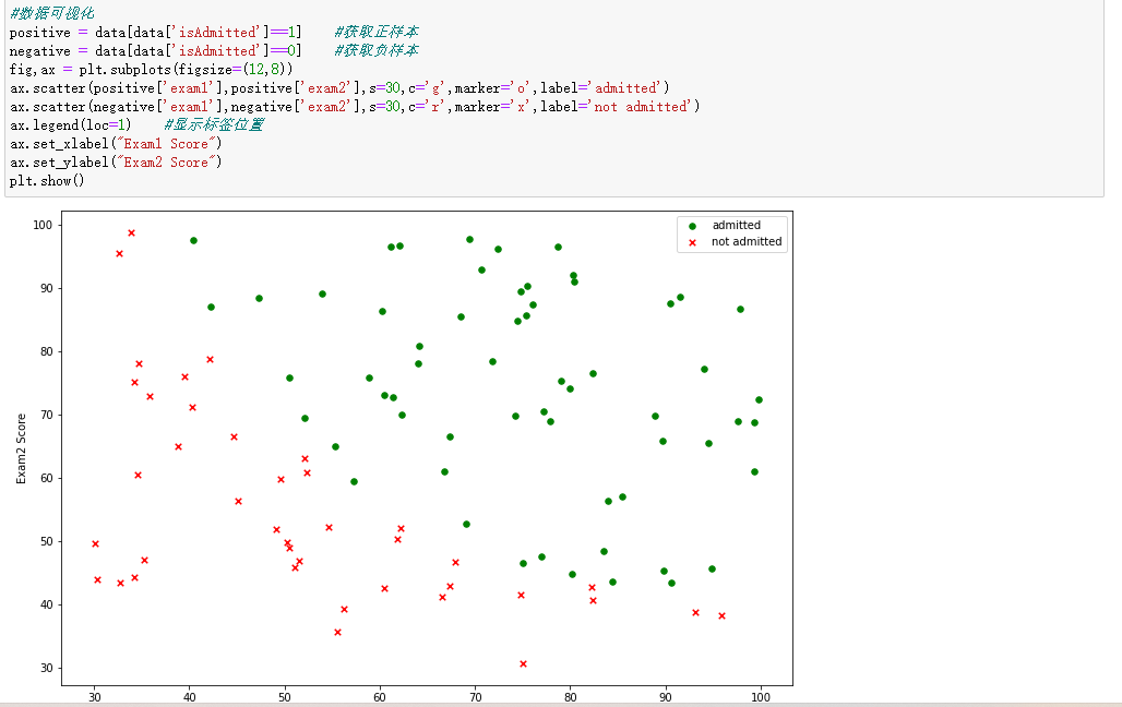
2.　数据可视化

#数据可视化
positive = data[data['isAdmitted']==1]    #获取正样本
negative = data[data['isAdmitted']==0]    #获取负样本
fig,ax = plt.subplots(figsize=(12,8))
ax.scatter(positive['exam1'],positive['exam2'],s=30,c='g',marker='o',label='admitted')
ax.scatter(negative['exam1'],negative['exam2'],s=30,c='r',marker='x',label='not admitted')
ax.legend(loc=1)    #显示标签位置
ax.set_xlabel("Exam1 Score")
ax.set_ylabel("Exam2 Score")
plt.show()

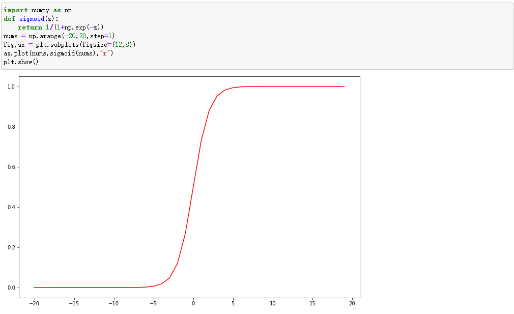
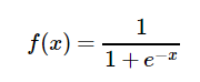
3.编写sigmoid函数代码

逻辑回归函数的定义为：

$h_{\theta}(x)=g(\theta^{T}x)$

逻辑回归函数为：

$h_{\theta}(x)=\frac{1}{1+e^{-\theta^{T}x}}$

import numpy as np
def sigmoid(z):
    return 1/(1+np.exp(-z))
nums = np.arange(-20,20,step=1)
fig,ax = plt.subplots(figsize=(12,8))
ax.plot(nums,sigmoid(nums),"r")
plt.show()

4.逻辑回归代价函数

def cost(theta, X, y):
    theta = np.matrix(theta)
    X = np.matrix(X)
    y = np.matrix(y)
    first = np.multiply(-y, np.log(sigmoid(X * theta.T)))
    second = np.multiply((1 - y), np.log(1 - sigmoid(X * theta.T)))
    return np.sum(first - second) / (len(X))
# 原始数据新建一列更易使用代价函数代码
data.insert(0, 'Ones', 1)
cols = data.shape[1]
X = data.iloc[:,0:cols-1]#训练集
y = data.iloc[:,cols-1:cols]#label
#转换numnp数组
X = np.array(X.values)
y = np.array(y.values)
theta = np.zeros(3)
X.shape, theta.shape, y.shape
cost(theta, X, y)

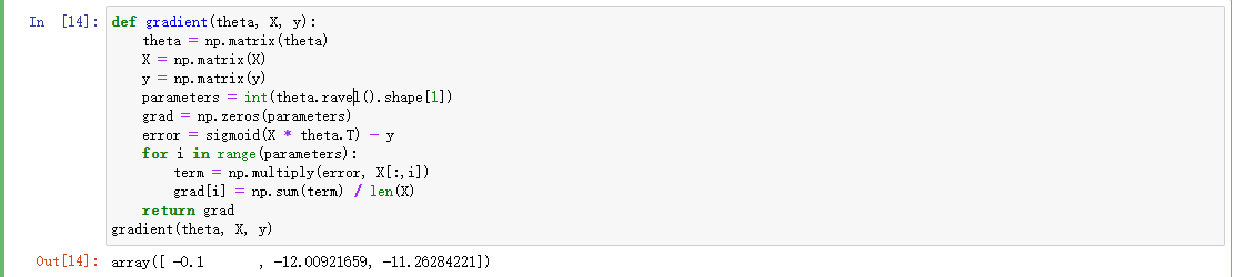
5.编写梯度函数代码

def gradient(theta, X, y):
theta = np.matrix(theta)
X = np.matrix(X)
y = np.matrix(y)
parameters = int(theta.ravel().shape[1])
grad = np.zeros(parameters)
error = sigmoid(X * theta.T) - y
for i in range(parameters):
term = np.multiply(error, X[:,i])
grad[i] = np.sum(term) / len(X)
return grad
gradient(theta, X, y)

6.编写寻找最优化参数代码

import scipy.optimize as opt
result = opt.fmin_tnc(func=cost, x0=theta, fprime=gradient, args=(X, y))
result

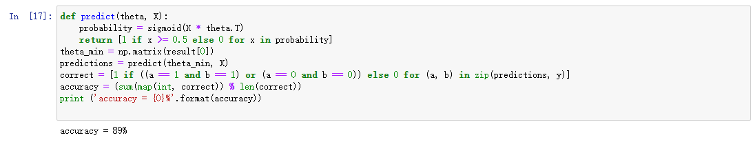
7.编写模型评估代码，输出准确率

def predict(theta, X):
    probability = sigmoid(X * theta.T)
    return [1 if x >= 0.5 else 0 for x in probability]
theta_min = np.matrix(result[0])
predictions = predict(theta_min, X)
correct = [1 if ((a == 1 and b == 1) or (a == 0 and b == 0)) else 0 for (a, b) in zip(predictions, y)]
accuracy = (sum(map(int, correct)) % len(correct))
print ('accuracy = {0}%'.format(accuracy))

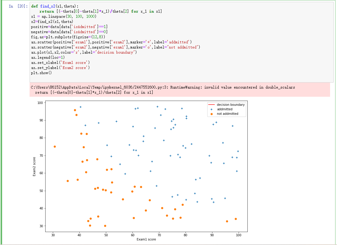
8.寻找决策边界，画出决策边界直线图

def find_x2(x1,theta):
return [(-theta[0]-theta[1]*x_1)/theta[2] for x_1 in x1]
x1 = np.linspace(30, 100, 1000)
x2=find_x2(x1,theta)

positive=data[data['isAdmitted']==1]
negative=data[data['isAdmitted']==0]
fig,ax=plt.subplots(figsize=(12,8))
ax.scatter(positive['exam1'],positive['exam2'],marker='+',label='addmitted')
ax.scatter(negative['exam2'],negative['exam1'],marker='o',label="not addmitted")
ax.plot(x1,x2,color='r',label="decision boundary")
ax.legend(loc=1)
ax.set_xlabel('Exam1 score')
ax.set_ylabel('Exam2 score')
plt.show()

问题二：

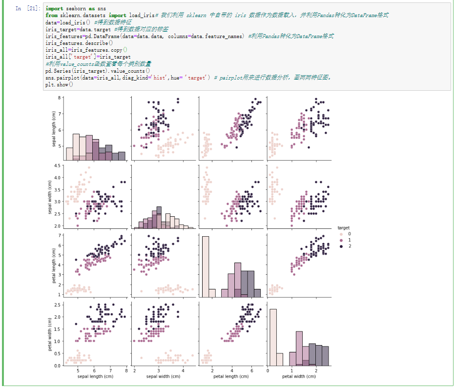
（1）使用seaborn库进行数据可视化

import seaborn as sns
from sklearn.datasets import load_iris# 我们利用 sklearn 中自带的 iris 数据作为数据载入，并利用Pandas转化为DataFrame格式
data=load_iris() #得到数据特征
iris_target=data.target #得到数据对应的标签
iris_features=pd.DataFrame(data=data.data, columns=data.feature_names) #利用Pandas转化为DataFrame格式
iris_features.describe()
iris_all=iris_features.copy()
iris_all['target']=iris_target
#利用value_counts函数查看每个类别数量
pd.Series(iris_target).value_counts()
sns.pairplot(data=iris_all,diag_kind='hist',hue= 'target') # pairplot用来进行数据分析，画两两特征图。
plt.show()

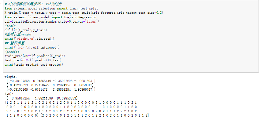
2.将iri数据集分为训练集和测试集(两者比例为8:2)进行三分类训练和预测

# 将训练集测试集按照8：2比例划分
from sklearn.model_selection import train_test_split
X_train,X_test,y_train,y_test = train_test_split(iris_features,iris_target,test_size=0.2)
from sklearn.linear_model import LogisticRegression
clf=LogisticRegression(random_state=0,solver='lbfgs')
#train
clf.fit(X_train,y_train)
#查看权重weight
print('wieght:\n',clf.coef_)
## 查看偏置
print('(w0):\n',clf.intercept_)
#predict
train_predict=clf.predict(X_train)
test_predict=clf.predict(X_test)
print(train_predict,test_predict)

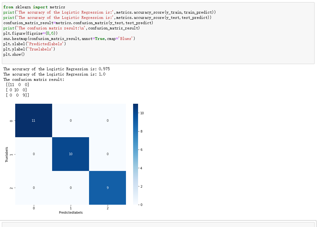
3.输出分类结果的混淆矩阵

from sklearn import metrics
print('The accuracy of the Logistic Regression is:',metrics.accuracy_score(y_train,train_predict))
print('The accuracy of the Logistic Regression is:',metrics.accuracy_score(y_test,test_predict))
confusion_matrix_result=metrics.confusion_matrix(y_test,test_predict)
print('The confusion matrix result:\n',confusion_matrix_result)
plt.figure(figsize=(8,6))
sns.heatmap(confusion_matrix_result,annot=True,cmap='Blues')
plt.xlabel('Predictedlabels')
plt.ylabel('Truelabels')
plt.show()