Logistic 回归

Logistic回归是目前最常用的一种分类算法。之前讨论了线性回归 http://www.cnblogs.com/futurehau/p/6105011.html，采用线性回归是不能解决或者说不能很好解决分类问题的，很直观的一个解释如下图所示，这里介绍Logistic回归。

一、Logistic 回归模型

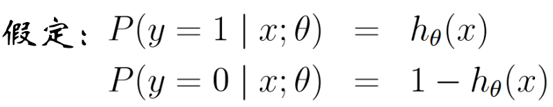
1.1 概率：

1.2 ML准则推导代价函数

1.2.1 y取1 0

似然函数：

对数似然函数及其求导：

1.2.2 y取 +1 -1

考虑到 1 - h(x) = h(-x)

似然函数可以表示为：

 

取对数变换可得：

最后得到：

 

 

 

1.3 代价函数：

在线性回归中，我们得到代价函数，但是在Logistic 回归中，由于h(x)是一个复杂的非线性函数，这就导致J(theta)变为一个非凸函数，梯度下降算法不能收敛到它的全局最小值，所以这里我们需要重新引入别的代价函数。

我们上文推到了似然函数为，那么我们这里取代价函数为似然函数的负，这样对于代价函数的最小化就相当于似然函数的最大化。我们不难得到下面的代价函数：

我们拆分开来看看是什么样子：

画出图来可以分析。如果 y= 1, 那么你预测 h(x) = 0 的代价就会非常高，预测h(x) = 1的代价就是 0。y = 0的情况同理。

 

二、Logistic回归的求解

2.1 梯度下降算法求解 Logistic

线性回归中我们提出两种方法来求解theta，解析法和梯度下降算法。在Logistic回归中，没有解析解，我们使用梯度下降算法来求解。

注意到这里是加号。其实上式既可以看为似然函数的正梯度上升，也可以把括号里面的负号拿出来之后变为损失函数的梯度下降。

2.2 梯度下降算法求解 Logistic 回归和求解线性回归的区别与联系。

我们发现，梯度下降算法求解Logistic回归和求解线性回归的梯度下降的式子形式上式一样的，区别在于两者的h(x)是不同的，那么这之中隐含什么东西呢？

我们现在考虑这样一个概念：

几率：一个事件的几率，是指该事件发生的概率与该事件不发生的概率的比值。

对数几率：几率取对数

所以，我们求几率如下：

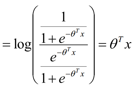
我们发现，Logistic的对数是线性的，这就相当于Logistic回归是一个广义的线性回归。对数线性模型。

三、决策边界

当h(x) 大于 0.5时，我们判决为1，小于0.5时，我们判决为假。接下来我们看看这意味着什么。

h(x) > 0.5 需要 theta * x > 0。当theta确定之后，这会得到关于x1,x2（只考虑二维）的一条曲线，把整个平面分为两部分，满足theta * x > 0的部分就取为1。

我们引入 theta * x = 0 为决策边界。决策边界和训练集没有关系，训练集是用来拟合参数theta的，theta确定之后，决策边界就确定了。

四、多元分类问题

4.1 使用多个二元 Logistic 回归分类器实现。

　　多次one Vs all，分别训练每个h(x)，分类的时候找出最大的那个h(x)。

4.2 SoftMax

理解还不是很清楚，关于这部分的一个解释：http://deeplearning.stanford.edu/wiki/index.php/Softmax%E5%9B%9E%E5%BD%92

4.3 多个二元分类 Vs SoftMax

如果你在开发一个音乐分类的应用，需要对k种类型的音乐进行识别，那么是选择使用 softmax 分类器呢，还是使用 logistic 回归算法建立 k 个独立的二元分类器呢？

这一选择取决于你的类别之间是否互斥，例如，如果你有四个类别的音乐，分别为：古典音乐、乡村音乐、摇滚乐和爵士乐，那么你可以假设每个训练样本只会被打上一个标签（即：一首歌只能属于这四种音乐类型的其中一种），此时你应该使用类别数 k = 4 的softmax回归。（如果在你的数据集中，有的歌曲不属于以上四类的其中任何一类，那么你可以添加一个“其他类”，并将类别数 k 设为5。）

如果你的四个类别如下：人声音乐、舞曲、影视原声、流行歌曲，那么这些类别之间并不是互斥的。例如：一首歌曲可以来源于影视原声，同时也包含人声 。这种情况下，使用4个二分类的 logistic 回归分类器更为合适。这样，对于每个新的音乐作品 ，我们的算法可以分别判断它是否属于各个类别。

现在我们来看一个计算视觉领域的例子，你的任务是将图像分到三个不同类别中。(i) 假设这三个类别分别是：室内场景、户外城区场景、户外荒野场景。你会使用sofmax回归还是 3个logistic 回归分类器呢？ (ii) 现在假设这三个类别分别是室内场景、黑白图片、包含人物的图片，你又会选择 softmax 回归还是多个 logistic 回归分类器呢？

在第一个例子中，三个类别是互斥的，因此更适于选择softmax回归分类器 。而在第二个例子中，建立三个独立的 logistic回归分类器更加合适。

 

鸢尾花lr代码

#!/usr/bin/python
# -*- coding:utf-8 -*-

import numpy as np
from sklearn.linear_model import LogisticRegression
import matplotlib.pyplot as plt
import matplotlib as mpl
from sklearn import preprocessing
import pandas as pd
from sklearn.preprocessing import StandardScaler
from sklearn.pipeline import Pipeline


def iris_type(s):
    it = {'Iris-setosa': 0, 'Iris-versicolor': 1, 'Iris-virginica': 2}
    return it[s]


if __name__ == "__main__":
    path = u'8.iris.data'  # 数据文件路径

    # # 手写读取数据
    # f = file(path)
    # x = []
    # y = []
    # for d in f:
    #     d = d.strip()
    #     if d:
    #         d = d.split(',')
    #         y.append(d[-1])
    #         x.append(map(float, d[:-1]))
    # print '原始数据X：\n', x
    # print '原始数据Y：\n', y
    # x = np.array(x)
    # print 'Numpy格式X：\n', x
    # y = np.array(y)
    # print 'Numpy格式Y - 1:\n', y
    # y[y == 'Iris-setosa'] = 0
    # y[y == 'Iris-versicolor'] = 1
    # y[y == 'Iris-virginica'] = 2
    # print 'Numpy格式Y - 2:\n', y
    # y = y.astype(dtype = np.int)
    # print 'Numpy格式Y - 3:\n', y
    #
    # # 使用sklearn的数据预处理
    # df = pd.read_csv(path, header=0)
    # x = df.values[:, :-1]
    # y = df.values[:, -1]
    # print 'x = \n', x
    # print 'y = \n', y
    #
    #
    # le = preprocessing.LabelEncoder()
    # le.fit(['Iris-setosa', 'Iris-versicolor', 'Iris-virginica'])
    #
    #
    # print le.classes_
    # y = le.transform(y)
    # print 'Last Version, y = \n', y
    #
    # # 路径，浮点型数据，逗号分隔，第4列使用函数iris_type单独处理
    data = np.loadtxt(path, dtype=float, delimiter=',', converters={4: iris_type})
    print data
    # 将数据的0到3列组成x，第4列得到y
    x, y = np.split(data, (4,), axis=1)

    # 为了可视化，仅使用前两列特征
    x = x[:, (2,3)]
    #
    print x
    print y
    #
    # x = StandardScaler().fit_transform(x) # 每一列数据标准化
    # lr = LogisticRegression()   # Logistic回归模型
    #     lr.fit(x, y.ravel())        # 根据数据[x,y]，计算回归参数
    #
    # 等价形式
    lr = Pipeline([('sc', StandardScaler()),
                        ('clf', LogisticRegression()) ])
    lr.fit(x, y.ravel()) # 转置

    # 画图
    N, M = 500, 500     # 横纵各采样多少个值
    x1_min, x1_max = x[:, 0].min(), x[:, 0].max()   # 第0列的范围
    x2_min, x2_max = x[:, 1].min(), x[:, 1].max()   # 第1列的范围
    t1 = np.linspace(x1_min, x1_max, N)
    t2 = np.linspace(x2_min, x2_max, M)
    x1, x2 = np.meshgrid(t1, t2)                    # 生成网格采样点
    x_test = np.stack((x1.flat, x2.flat), axis=1)   # 测试点

    # 无意义，只是为了凑另外两个维度
    # x3 = np.ones(x1.size) * np.average(x[:, 2])
    # x4 = np.ones(x1.size) * np.average(x[:, 3])
    # x_test = np.stack((x1.flat, x2.flat, x3, x4), axis=1)  # 测试点

    cm_light = mpl.colors.ListedColormap(['#77E0A0', '#FF8080', '#A0A0FF'])
    cm_dark = mpl.colors.ListedColormap(['g', 'r', 'b'])
    y_hat = lr.predict(x_test)                  # 预测值
    y_hat = y_hat.reshape(x1.shape)                 # 使之与输入的形状相同
    plt.pcolormesh(x1, x2, y_hat, cmap=cm_light)     # 预测值的显示
    plt.scatter(x[:, 0], x[:, 1], c=y, edgecolors='k', s=50, cmap=cm_dark)    # 样本的显示
    plt.xlabel('petal length')
    plt.ylabel('petal width')
    plt.xlim(x1_min, x1_max)
    plt.ylim(x2_min, x2_max)
    plt.grid()
    plt.savefig('2.png')
    plt.show()

    # 训练集上的预测结果
    y_hat = lr.predict(x)
    y = y.reshape(-1)
    result = y_hat == y
    print y_hat
    print result
    acc = np.mean(result)
    print '准确度: %.2f%%' % (100 * acc)

 SGD BGD:

# -*- coding: cp936 -*-
import numpy as np
import matplotlib.pyplot as plt
import math
def logestic_regression_SGD(x, y, alpha, lamda):
    m = np.alen(x)
    ones = np.ones(m)
    x = np.column_stack((ones, x))
    n = np.alen(x[0])
    theta = np.ones(n)
    for j in range(1, m):
        hypothesis = getHypothesis(x[j], theta)

        loss = hypothesis - y[j]
        print np.sum(loss ** 2)
        gradient = np.dot(loss, x[j])
        theta = theta - alpha * gradient
    return theta

def logestic_regression_BGD(x, y, alpha, lamda):
    m = np.alen(x)
    ones = np.ones(m)
    x = np.column_stack((ones, x))
    n = np.alen(x[0])
    theta = np.ones(n)
    x_traverse = np.transpose(x)

    for i in range(100000):
        hypothesis = getHypothesis(x, theta)
        loss = hypothesis - y
        # print np.sum(loss ** 2)
        gradient = np.dot(x_traverse, loss)
        theta = theta - alpha * gradient
    return theta

def getHypothesis(x, theta):
    return 1 / (1 + pow(math.e, -np.dot(x, theta)))


def generateData():
    x1 = (np.random.random_sample(500) - 0.5) * 2
    x2 = (np.random.random_sample(500) - 0.5) * 2
    y = (x1 ** 2 + x2 ** 2) <= 0.25
    x1_pos = []
    x1_neg = []
    x2_pos = []
    x2_neg = []
    len = np.alen(y)
    for i in range(len):
        if y[i]:
            x1_pos.append(x1[i])
            x2_pos.append(x2[i])
        else:
            x1_neg.append(x1[i])
            x2_neg.append(x2[i])
    plt.plot(x1_neg, x2_neg, 'rx')
    plt.plot(x1_pos, x2_pos, 'bo')
    plt.show()
    x1 = np.column_stack((x1, x1 * x1))
    x2 = np.column_stack((x2, x2 * x2))
    return [x1, x2, y]
if __name__ == '__main__':
    [x1, x2, y] = generateData()
    x = np.column_stack((x1, x2))
    theta = logestic_regression_SGD(x, y, 0.001, 0.01)
    print theta
    theta = logestic_regression_BGD(x, y, 0.01, 0.01)
    print theta