单应性Homograph估计
单应性Homograph估计
单应性原理被广泛应用于图像配准,全景拼接,机器人定位SLAM,AR增强现实等领域。这篇文章从基础图像坐标知识系为起点,讲解图像变换与坐标系的关系,介绍单应性矩阵计算方法,并分析深度学习在单应性方向的进展。
图像变换与平面坐标系的关系
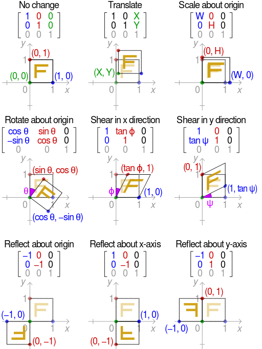
旋转
将图形围绕原点\((0,0)\)逆时针方向旋转\(\theta\)角,用解析式表示为:
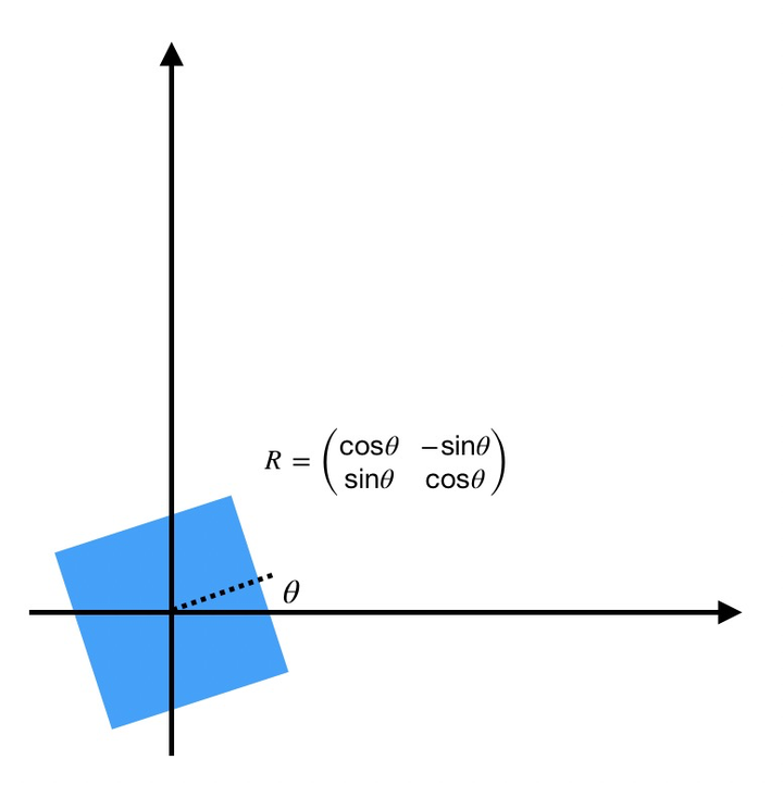
写成矩阵乘法形式:
平移
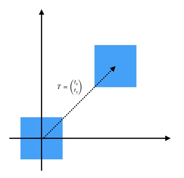
但是现在遇到困难了,平移无法写成和上面旋转一样的矩阵乘法形式。所以引入齐次坐标 \((x,y)\Leftrightarrow\),再写成矩阵形式:
其中\(I_{2\times 2}=\begin{bmatrix}1&0\\0&1\end{bmatrix}\)表示单位矩阵,而\(T_{2\times 1}=\begin{bmatrix}t_x\\t_y\end{bmatrix}\)表示平移向量。
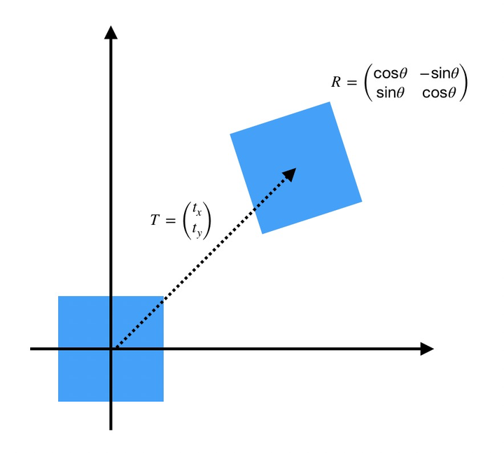
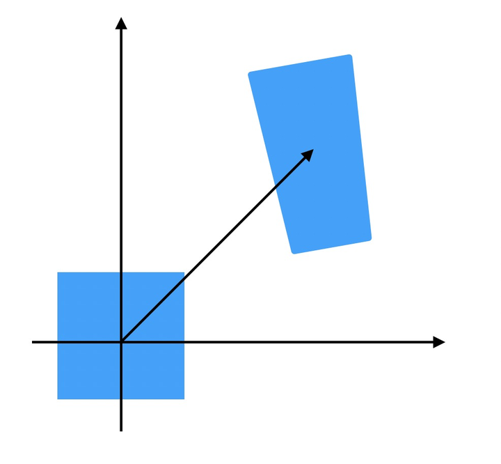
刚体变换
那么就可以把把旋转和平移统一写在一个矩阵乘法公式中,即刚体变换:
而旋转矩阵\(R_{2\times 2}\)是正交矩阵\((RR^T=R^TR=I)\)
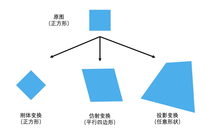
仿射变换
其中\(A_{2\times 2}=\begin{bmatrix}a_{11}&a_{12}\\a_{21}&a_{22}\end{bmatrix}\)可以是任意\(2\times 2\)矩阵,而\(R\)必须是正交矩阵
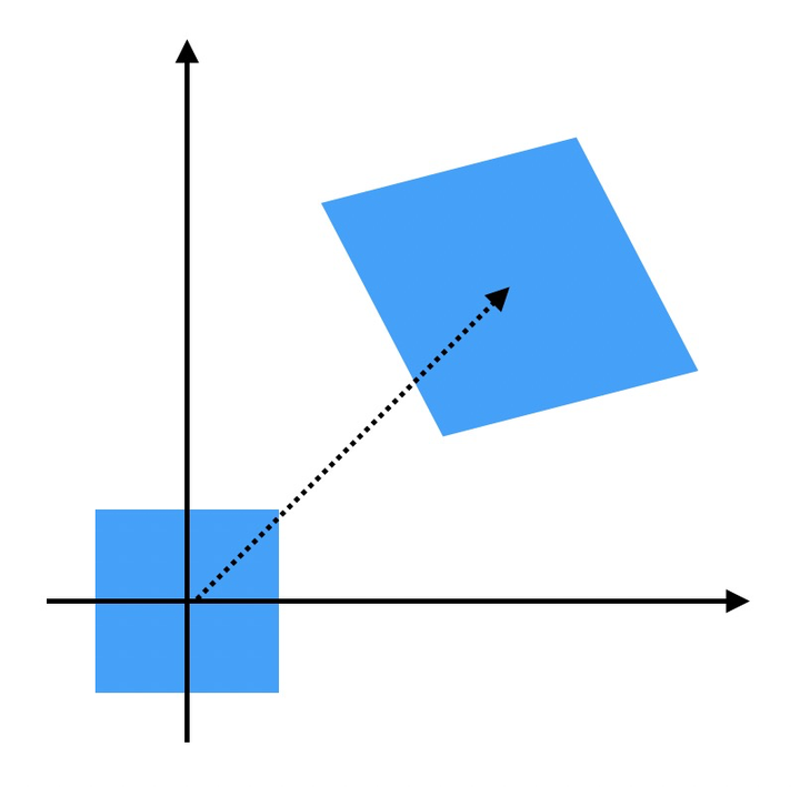
可以看到,相比刚体变换(旋转和平移),仿射变换除了改变目标位置,还改变目标的形状,但是会保持物体的“平直性(如图形中平行的两条线变换后依然平行)”。
不同\(A\)和\(T\)矩阵对应的各种基本仿射变换:
投影变换(单应性变换)
简单说,投影变换彻底改变目标的形状。
总结
- 刚体变换:平移+旋转,只改变物体位置,不改变物体形状
- 仿射变换:改变物体位置和形状,但是保持“平直性”(原来平行的边依然平行)
- 投影变换:彻底改变物体位置和形状
我们来看看完整投影变换矩阵各个参数的物理含义:
其中\(A_{2\times 2}\)代表仿射变换参数,\(T_{1\times 1}\)代表平移变换参数。
而\(V^T=[v_1,v_2]\)表示一种“变换后边缘交点”关系,如:
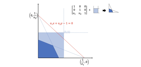
至于\(s\)则是一个与\(V^T=[v_1.v_2]\)相关的缩放因子。
一般情况下都会通过归一化使得\(s=1\),原因见下文。
平面坐标系与齐次坐标系
问题来了,齐次坐标到底是什么?
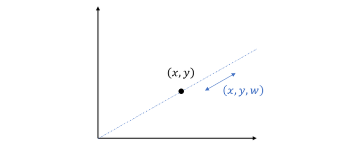
齐次坐标系\((x,y,w)\in \mathbb{P}^3\)与常见的三维空间坐标系\((x,y,z)\in \mathbb{R}^3\)不同,只有两个自由度:
而\(w\)(其中\(w>0\))对应坐标\(x\)和\(y\)的缩放尺度。当\(w=1\)时:
特别的当\(w=0\)时,对应无穷远:
从二维平面上看,\((x,y,w)\)随\(w\)的变化在从原点到\((x,y)\)的蓝虚线示意的射线上滑动:
单应性变换
单应性是什么?
此处给出单应性不严谨的定义:用 [无镜头畸变] 的相机从不同位置拍摄 [同一平面物体] 的图像之间存在单应性,可以用 [投影变换] 表示 。
单应变换就是投影变换,逆投影变换是投影变换的逆
注意:
单应性的严格定义与成立条件非常复杂,超出本文范围。
有需要的朋友请自行查阅《Multiple View Geometry in Computer Vision》书中相关内容。
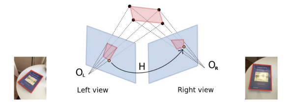
简单说就是:
其中\((x_l,y_l)\)是Left view图片上的点,\((x_r,y_r)\)是Right view图片上对应的点。
那么这个\(H_{3\times3}\)单应性矩阵如何求解呢?
从更一般的情况分析,每一组匹配点\((x_i,y_i)\overset{match}{\longrightarrow}(x_i',y_i')\)有以下等式成立:
由平面坐标与齐次坐标对应关系\((\frac{x}{w},\frac{y}{w})\in \mathbb{R}^2\Leftrightarrow (x,y,w)\in \mathbb{P}^3\),上式可以表示为:
\(\begin{matrix}x'_i=\frac{h_{11}x_i+h_{12}y_i+h_{13}}{h_{31}x_i+h_{32}y_i+h_{33}}\\y'_i=\frac{h_{21}x_i+h_{22}y_i+h_{23}}{h_{31}x_i+h_{32}y_i+h_{33}}\end{matrix}\)
进一步变换为:
写成矩阵\(AX=0\)形式:
也就是说一组匹配点\((x_i,y_i)\overset{match}{\longrightarrow}(x_i',y_i')\)可以获得2组方程。
单应性矩阵8自由度
注意观察:单应性矩阵\(H\)与\(aH\)其实是完全一样的(其中$a\ne 0 $),例如:
即点\((x_i,y_i)\)无论经过\(H\)还是\(aH\)映射,变化后都是\((x_i',y_i')\)。
如果使\(a=\frac{1}{h_{33}}\),那么有:
所以单应性矩阵\(H\)虽然有9个未知数,但是只有8个自由度。
在求\(H\)时一般添加约束\(h_{33}=1\)(也有用\(\sqrt{h_{11}^2+h_{12}^2+...+h_{33}^2}=1\)约束),所以还有\(h_{11}\sim h_{32}\)共8个未知数。由于一组匹配点\((x_i,y_i)\overset{match}{\longrightarrow}(x_i',y_i')\)对应2组方程,那么只需要\(n=4\)组不共线的匹配点即可求解\(H\)的唯一解。
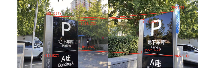
下图为xiaomi9拍摄,有镜头畸变:
OpenCV已经提供了相关API,代码和变换结果如下。
import cv2
import numpy as np

im1 = cv2.imread('left.jpg')
im2 = cv2.imread('right.jpg')

src_points = np.array([[581, 297], [1053, 173], [1041, 895], [558, 827]])
dst_points = np.array([[571, 257], [963, 333], [965, 801], [557, 827]])

H, _ = cv2.findHomography(src_points, dst_points)

h, w = im2.shape[:2]

im2_warp = cv2.warpPerspective(im2, H, (w, h))
可以看到:
- 红框所在平面上内容基本对齐,但受到镜头畸变影响无法完全对齐;
- 平面外背景物体不符合单应性原理,偏离很大,完全无法对齐。
传统方法估计单应性矩阵
一般传统方法估计单应性变换矩阵,需要经过以下4个步骤:
- 提取每张图SIFT/SURF/FAST/ORB等特征点
- 提取每个特征点对应的描述子
- 通过匹配特征点描述子,找到两张图中匹配的特征点对(这里可能存在错误匹配)
- 使用RANSAC算法剔除错误匹配
- 求解方程组,计算Homograph单应性变换矩阵
示例代码如下:
#coding:utf-8

# This code only tested in OpenCV 3.4.2!
import cv2
import numpy as np

# 读取图片
im1 = cv2.imread('left.jpg')
im2 = cv2.imread('right.jpg')

# 计算SURF特征点和对应的描述子,kp存储特征点坐标,des存储对应描述子
surf = cv2.xfeatures2d.SURF_create()
kp1, des1 = surf.detectAndCompute(im1, None)
kp2, des2 = surf.detectAndCompute(im2, None)

# 匹配特征点描述子
bf = cv2.BFMatcher()
matches = bf.knnMatch(des1, des2, k=2)

# 提取匹配较好的特征点
good = []
for m,n in matches:
    if m.distance < 0.7*n.distance:
        good.append(m)

# 通过特征点坐标计算单应性矩阵H
# (findHomography中使用了RANSAC算法剔初错误匹配)
src_pts = np.float32([kp1[m.queryIdx].pt for m in good]).reshape(-1,1,2)
dst_pts = np.float32([kp2[m.trainIdx].pt for m in good]).reshape(-1,1,2)
H, mask = cv2.findHomography(src_pts, dst_pts, cv2.RANSAC, 5.0)
matchesMask = mask.ravel().tolist()

# 使用单应性矩阵计算变换结果并绘图
h, w, d = im1.shape
pts = np.float32([[0,0], [0,h-1], [w-1,h-1], [w-1,0]]).reshape(-1,1,2)
dst = cv2.perspectiveTransform(pts, H)
img2 = cv2.polylines(im2, [np.int32(dst)], True, 255, 3, cv2.LINE_AA)

draw_params = dict(matchColor = (0,255,0), # draw matches in green color
                   singlePointColor = None,
                   matchesMask = matchesMask, # draw only inliers
                   flags = 2)

im3 = cv2.drawMatches(im1, kp1, im2, kp2, good, None, **draw_params)
相关内容网上资料较多,这里不再重复造轮子。需要说明,一般情况计算出的匹配的特征点对\((x_i,y_i)\overset{match}{\longrightarrow}(x_i',y_i')\)数量都有\(n \gg 4\),此时需要解超定方程组(类似于求解线性回归时数据点的数量远多于未知数)。
深度学习在单应性方向的进展
HomographyNet(深度学习end2end估计单应性变换矩阵)
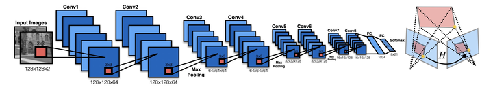
HomographyNet是发表在CVPR 2016的一种用深度学习计算单应性变换的网络,即输入两张图,直接输出单应性矩阵\(H\)。
在之前的分析中提到,只要有4组\((x_i,y_i)\overset{match}{\longrightarrow}(x_i',y_i')\)匹配点即可计算\(H_{3\times 3}\)的唯一解。
相似的,只要有4组\((\bigtriangleup x_i,\bigtriangleup y_i)\)也可以计算出\(H_{3\times 3}\)的唯一解:
其中\(\bigtriangleup x_i=x_i-x_i'\)且\(\bigtriangleup y_i=y_i-y_i'\)
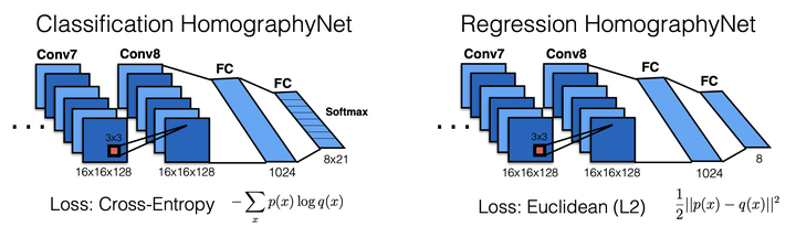
分析到这里,如果要计算\(H\),网络输出可以有以下2种情况:
-
Regression:网络直接输出\((\bigtriangleup x_1,\bigtriangleup y_1)\sim (\bigtriangleup x_4,\bigtriangleup y_4)\)共8个数值
这样设置网络非常直观,使用L2损失训练,测试时直接输出8个float values,但是没有置信度confidence。即在使用网络时,无法知道当前输出单应性可靠程度。
-
Classification:网络输出\((\bigtriangleup x_1,\bigtriangleup y_1)\sim (\bigtriangleup x_4,\bigtriangleup y_4)\)共8个数值的量化值+confidence
这时将网络输出每个\(\bigtriangleup x_i\)和\(\bigtriangleup y_i\)量化成21个区间,用分类的方法判断落在哪一个区间。训练时使用Softmax损失。相比回归直接输出数值,量化必然会产生误差,但是能够输出分类置信度评判当前效果好坏,更便于实际应用。
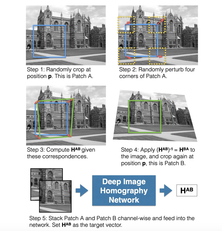
另外HomographyNet训练时数据生成方式也非常有特色。
- 首先在随机\(p\)位置获取正方形图像块Patch A
- 然后对正方形4个点进行随机扰动,同时获得4组\((\bigtriangleup x_i,\bigtriangleup y_i)\)
- 再通过4组\((\bigtriangleup x_i,\bigtriangleup y_i)\)计算\(H^{AB}\)
- 最后将图像通过\(H^{AB}=(H^{AB})^{-1}\)变换,在变换后图像\(p\)位置获取正方形图像块Patch B
那么图像块A和图像块B作为输入,4组\((\bigtriangleup x_i,\bigtriangleup y_i)\)作为监督Label,进行训练
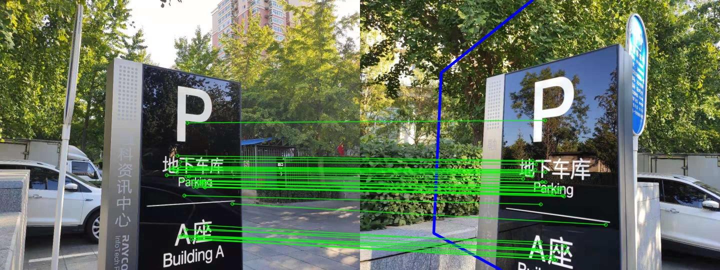
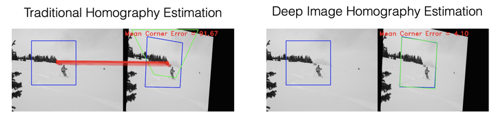
可以看到,在无法提取足够特征点的弱纹理区域,HomographyNet相比传统方法确实有一定的优势:
Spatial Transformer Networks(直接对CNN中的卷积特征进行变换)
其实早在2015年,就已经有对CNN中的特征进行变换的STN结构。
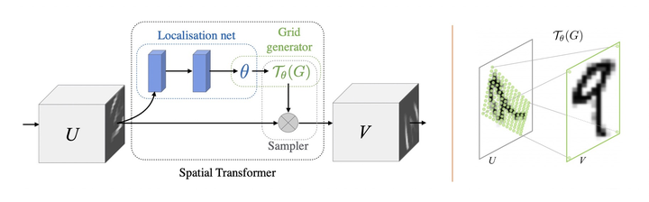
假设有特征层\(U\),经过卷积变为\(V\),可以在他们之间插入STN结构。这样就可以直接学习到从特征\(U\)上的点\((\bigtriangleup x_i^u,\bigtriangleup y_i^u)\)的仿射变换。
其中\(A_\theta\)对应STN中的仿射变换参数。STN直接在特征维度进行变换,且可以插入轻松任意两层卷积中。
DELF: DEep Local Features(深度学习提取特征点与描述子)
之前提到传统方法使用SIFT和Surf等特征点估计单应性。显然单应性最终估计准确度严重依赖于特征点和描述子性能。Google在ICCV 2017提出使用使用深度学习提取特征点。
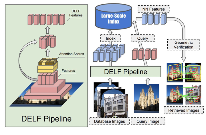
考虑到篇幅,这里不再展开DELF,请有兴趣的读者自行了解相关内容。
关于OpenCV图像坐标系的问题
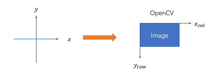
需要说明的是,在上述分析中使用的是\((x,y)\)坐标系,但是在OpenCV等常用图像库中往往使用图像左上角为原点的\((x_{col},y_{row})\)的像素坐标系,会导致OpenCV中的Homograph矩阵与上述推导有一些差异。
本文来自博客园,作者:甫生,转载请注明原文链接:https://www.cnblogs.com/fusheng-rextimmy/p/15466520.html