day03:matplotlib
导入相关包
In [ ]:
import pandas as pd
import matplotlib.pyplot as plt

# 中文乱码的处理
plt.rcParams['font.sans-serif']=['PingFang HK'] #mac系统使用
# plt.rcParams['font.sans-serif'] = ['Microsoft YaHei']# windows使用设置微软雅黑字体
plt.rcParams['axes.unicode_minus'] = False # 避免坐标轴不能正常的显示负号
线图:plot()
- 函数功能:展现变量的变化趋势
- 调用方法:plt.plot(x, y, linestyle, linewidth,color,marker, markersize, markeredgecolor, markerfactcolor, label, alpha)
- x:指定折线图的x轴数据;
- y:指定折线图的y轴数据;
- linestyle:指定折线的类型,可以是实线、虚线、点虚线、点点线等,默认文实线;
- linewidth:指定折线的宽度
- marker:可以为折线图添加点,该参数是设置点的形状;
- markersize:设置点的大小;
- markeredgecolor:设置点的边框色;
- markerfactcolor:设置点的填充色;
- label:为折线图添加标签,类似于图例的作用;
- 画一个直线
In [ ]:
x1 = [1,2,3,4,5]
y1 = [4,5,6,7,8]
plt.plot(x1,y1)
Out[ ]:
[<matplotlib.lines.Line2D at 0x127db8370>]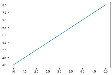
- 画一个抛物线
In [ ]:
x2 = pd.Series([1,2,3,4,5])
y2 = x2 ** 4

plt.plot(x2,y2)
Out[ ]:
[<matplotlib.lines.Line2D at 0x132951ca0>]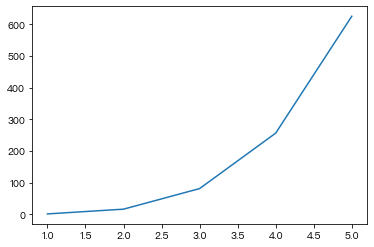
- 用点加虚线的方式画出x=(0,10)间sin的图像
-
其他line的属性:如color,linestyle,linewidth,marker,可参考以下资料:https://blog.csdn.net/dss_dssssd/article/details/84430024
-
In [ ]:
plt.plot(x2,y2,c='green',alpha=0.6)Out[ ]:
[<matplotlib.lines.Line2D at 0x13298ceb0>]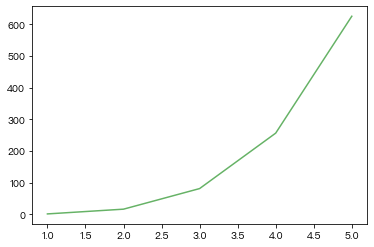
- 给上图添加图例
- 使用label参数结合这legend方法
In [ ]:
plt.plot(x1,y1,label='ret1')
plt.plot(x2,y2,label='ret2')
plt.legend()
Out[ ]:
<matplotlib.legend.Legend at 0x133438c10>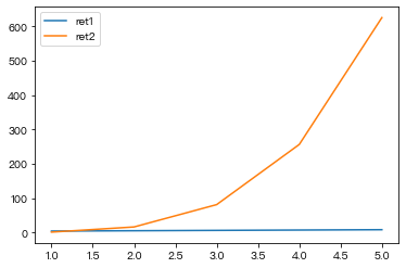
- 没有线性关系的两组数据的折线图
In [ ]:
x = [3,6,8,2,1]
y = [9,5,6,1,2]

plt.plot(x,y)
Out[ ]:
[<matplotlib.lines.Line2D at 0x1334a14f0>]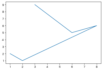
- 调整图例的大小比例
In [ ]:
plt.figure(figsize=(8,10))

plt.plot(x1,y1,label='ret1')
plt.plot(x2,y2,label='ret2')
plt.legend()
Out[ ]:
<matplotlib.legend.Legend at 0x1335502e0>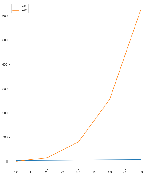
散点图
- 函数功能:散点图,寻找变量之间的关系
- 调用方法:plt.scatter(x, y, s, c, marker, cmap, norm, alpha, linewidths, edgecolorsl)
- 参数说明:
- x: x轴数据
- y: y轴数据
- s: 散点大小
- c: 散点颜色
- marker: 散点图形状
- cmap: 指定某个colormap值,该参数一般不用,用默认值
- alpha: 散点的透明度
- linewidths: 散点边界线的宽度
- edgecolors: 设置散点边界线的颜色
- 绘制两组100个随机数的散点图
In [ ]:
import numpy as np
x1 = np.random.randint(0,100,size=(30,))
y1 = np.random.randint(0,100,size=(30,))
In [ ]:
plt.scatter(x1,y1)Out[ ]:
<matplotlib.collections.PathCollection at 0x1335beac0>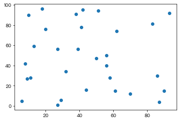
In [ ]:
x1 = x1
y1 = x1 ** 2

plt.scatter(x1,y1)
Out[ ]:
<matplotlib.collections.PathCollection at 0x134af85e0>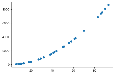
条形图:bar(), barh()
- 调用方法:plt.bar(x, y, width,color, edgecolor, bottom, linewidth, align, tick_label, align)
- 参数说明:
- x:指定x轴上数值
- y:指定y轴上的数值
- width:表示条形图的宽度,取值在0~1之间,默认为0.8
- color:条形图的填充色
- edgecolor:条形图的边框颜色
- bottom:百分比标签与圆心距离
- linewidth:条形图边框宽度
- tick_label:条形图的刻度标签
- align:指定x轴上对齐方式,"center","edge"边缘
- 简单垂直条形图
In [ ]:
GDP = [36102,38700,14083,25002]
city = ['北京','上海','天津','重庆']

plt.bar(city,GDP)
Out[ ]:
<BarContainer object of 4 artists>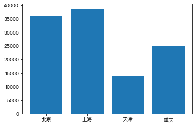
In [ ]:
plt.barh(city,GDP)Out[ ]:
<BarContainer object of 4 artists>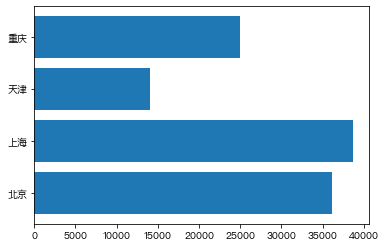
In [ ]:
#给图像添加相关的标识
GDP = [36102,38700,14083,25002]
city = ['北京','上海','天津','重庆']

plt.bar(city,GDP)

plt.xlabel('城市名称')
plt.ylabel('城市GDP')
plt.title('城市&GDP')
Out[ ]:
Text(0.5, 1.0, '城市&GDP')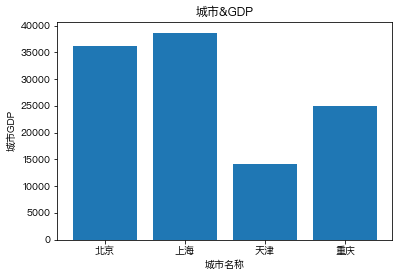
饼图
- 函数功能:表示离散变量各水平占比情况
- 参数说明:
- x:指定绘图的数据
- explode:指定饼图某些部分的突出显示,即呈现爆炸式
- labels:为饼图添加标签说明,类似于图例说明
- colors:指定饼图的填充色
- autopct:自动添加百分比显示,可以采用格式化的方法显示
- pctdistance:设置百分比标签与圆心的距离
- shadow:是否添加饼图的阴影效果
- labeldistance:设置各扇形标签(图例)与圆心的距离;
- startangle:设置饼图的初始摆放角度;
- radius:设置饼图的半径大小;
- counterclock:是否让饼图按逆时针顺序呈现;
- wedgeprops:设置饼图内外边界的属性,如边界线的粗细、颜色等;
- textprops:设置饼图中文本的属性,如字体大小、颜色等;
- center:指定饼图的中心点位置,默认为原点
- frame:是否要显示饼图背后的图框,如果设置为True的话,需要同时控制图框x轴、y轴的范围和饼图的中心位置;
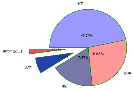
- 为饼图添加一些参数
In [ ]:
#构造数据:某城镇受教育程度
education = [9823, 5601, 3759, 1400, 450]
labels = ['小学', '初中', '高中', '大学', '研究生及以上']

explode = [0,0,0,0.6,0.8]  # 用于突出显示特定人群
colors=['#9999ff','#ff9999','#7777aa','#2442aa','#dd5555'] # 自定义颜色


# 绘制饼图
a = plt.pie(x = education, # 绘图数据
        explode=explode, # 分割部分距离圆心的距离
        labels=labels, # 添加教育水平标签
        colors=colors, # 设置饼图的自定义填充色
        autopct='%.2f%%', # 设置百分比的格式,这里保留一位小数
        pctdistance=0.3,  # 设置百分比标签与圆心的距离
        labeldistance = 1.15, # 设置教育水平标签与圆心的距离
        startangle = 180, # 设置饼图的初始角度
        radius = 1.5, # 设置饼图的半径
        counterclock = False, # 是否逆时针,这里设置为顺时针方向
        wedgeprops = {'linewidth': 1.5, 'edgecolor':'green'},# 设置饼图内外边界的属性值
        textprops = {'fontsize':12, 'color':'k'}, # 设置文本标签的属性值
        )
图像的保存
In [ ]:
#1.创建一个figure对象
fig = plt.figure()

#2.画图代码
plt.pie(x=[3,8,5,7,6])

#3.保存图片
fig.savefig('pie.png')
直方图/密度图:hist()
- 函数功能:判定数据的分布情况
- 参数说明:
- x:指定要绘制直方图的数据;
- bins:指定直方图条形的个数;
- range:指定直方图数据的上下界,默认包含绘图数据的最大值和最小值;
- density:是否将直方图的频数转换成频率;
- weights:该参数可为每一个数据点设置权重;
- cumulative:是否需要计算累计频数或频率;
- bottom:可以为直方图的每个条形添加基准线,默认为0;
- histtype:指定直方图的类型,默认为bar,除此还有’barstacked’, ‘step’, ‘stepfilled’;
- align:设置条形边界值的对其方式,默认为mid,除此还有’left’和’right’;
- orientation:设置直方图的摆放方向,默认为垂直方向;
- rwidth:设置直方图条形宽度的百分比;
- log:是否需要对绘图数据进行log变换;
- color:设置直方图的填充色;
- label:设置直方图的标签,可通过legend展示其图例;
- stacked:当有多个数据时,是否需要将直方图呈堆叠摆放,默认水平摆放;
- 绘制简单频数直方图
In [ ]:
data = [1,1,2,2,3,3,3,3,3,3,4,5,6,6]
plt.hist(x=data,bins=10)
Out[ ]:
(array([2., 0., 2., 0., 6., 0., 1., 0., 1., 2.]),
 array([1. , 1.5, 2. , 2.5, 3. , 3.5, 4. , 4.5, 5. , 5.5, 6. ]),
 <BarContainer object of 10 artists>)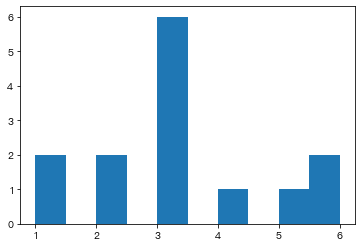
- hist()函数会返回三组结果:
- 返回值1:原始数据在不同区间存在的元素个数
- 返回值2:表示每根柱子对应的数值区间
- 返回值3:直方图图像
分析目的
- 通过分析销售数据来了解某在线销售平台的销售情况,基于用户消费数据来分析店铺的销售情况和用户的消费行为。
- 基于店铺的销售情况,我们想主要了解:
- 每月的销售金额
- 每月的消费人数
- 每月的订单数量
- 不同省份的用户数量
- 不同省份的订单数量
- 不同省份的成交金额
- 基于用户的消费行为,我们想主要了解:
- 用户消费次数
- 用户消费金额
- 用户消费次数和消费金额的关系
- 新老用户的占比
数据加载
In [ ]:
import pandas as pd
import matplotlib.pyplot as plt

# 中文乱码的处理
plt.rcParams['font.sans-serif']=['PingFang HK'] #mac系统使用
In [ ]:
#数据加载   ../data/data.csv
df = pd.read_csv('../data/data.csv').drop(columns='Unnamed: 0')
df.head()
Out[ ]:
| 订单编号 | 类别 | 品牌 | 价格 | 用户编号 | 年龄 | 性别 | 省份 | 下单日期 | 下单小时 | 下单月份 | |
|---|---|---|---|---|---|---|---|---|---|---|---|
| 0 | 2294359932054536986 | electronics.tablet | samsung | 162.01 | 1515915625441993984 | 24.0 | 女 | 海南 | 2020-04-24 | 11 | 2020-04-01 |
| 1 | 2294444024058086220 | electronics.audio.headphone | huawei | 77.52 | 1515915625447879424 | 38.0 | 女 | 北京 | 2020-04-24 | 14 | 2020-04-01 |
| 2 | 2294584263154074236 | 2268105471367840000 | karcher | 217.57 | 1515915625443148032 | 32.0 | 女 | 广东 | 2020-04-24 | 19 | 2020-04-01 |
| 3 | 2295716521449619559 | furniture.kitchen.table | maestro | 39.33 | 1515915625450382848 | 20.0 | 男 | 重庆 | 2020-04-26 | 8 | 2020-04-01 |
| 4 | 2295740594749702229 | electronics.smartphone | apple | 1387.01 | 1515915625448766464 | 21.0 | 男 | 北京 | 2020-04-26 | 9 | 2020-04-01 |
In [ ]:
df.shapeOut[ ]:
(365427, 11)数据分析
店铺销售情况分析
- 查看店铺每月的销售金额
In [ ]:
price_ret = df.groupby(by='下单月份')['价格'].sum()
price_ret
Out[ ]:
下单月份
2020-01-01     1729464.93
2020-02-01     2216672.31
2020-03-01     2841015.58
2020-04-01     1669080.19
2020-05-01     7642033.70
2020-06-01     7486587.13
2020-07-01    16019435.00
2020-08-01    27361373.12
2020-09-01    15143005.10
Name: 价格, dtype: float64
In [ ]:
plt.plot(price_ret.index,price_ret.values)
plt.xticks(rotation=30)
Out[ ]:
([0, 1, 2, 3, 4, 5, 6, 7, 8],
 [Text(0, 0, ''),
  Text(0, 0, ''),
  Text(0, 0, ''),
  Text(0, 0, ''),
  Text(0, 0, ''),
  Text(0, 0, ''),
  Text(0, 0, ''),
  Text(0, 0, ''),
  Text(0, 0, '')])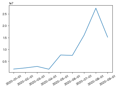
- 查看店铺每月的消费人数
In [ ]:
users_ret = df.groupby(by='下单月份')['用户编号'].count()
users_ret
Out[ ]:
下单月份
2020-01-01    13449
2020-02-01    16948
2020-03-01    17667
2020-04-01    11332
2020-05-01    38570
2020-06-01    39114
2020-07-01    73244
2020-08-01    95976
2020-09-01    59127
Name: 用户编号, dtype: int64
In [ ]:
plt.plot(users_ret.index,users_ret.values)
plt.xticks(rotation=30)
Out[ ]:
([0, 1, 2, 3, 4, 5, 6, 7, 8],
 [Text(0, 0, ''),
  Text(0, 0, ''),
  Text(0, 0, ''),
  Text(0, 0, ''),
  Text(0, 0, ''),
  Text(0, 0, ''),
  Text(0, 0, ''),
  Text(0, 0, ''),
  Text(0, 0, '')])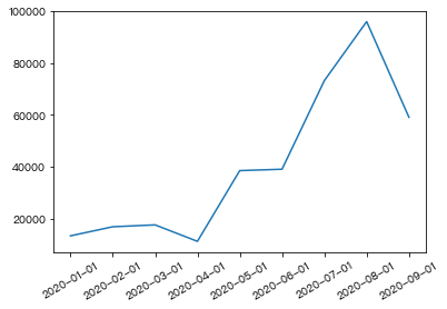
- 每月订单数量
In [ ]:
df.groupby(by='下单月份').size()Out[ ]:
下单月份
2020-01-01    13449
2020-02-01    16948
2020-03-01    17667
2020-04-01    11332
2020-05-01    38570
2020-06-01    39114
2020-07-01    73244
2020-08-01    95976
2020-09-01    59127
dtype: int64- 不同省份的用户数量
In [ ]:
s1 = df.groupby(by='省份')['用户编号'].nunique().sort_values()
s1
Out[ ]:
省份
湖南     4766
天津     4784
湖北     4787
浙江     4791
重庆     4803
四川     4872
海南     4901
江苏     4953
北京    14306
上海    14430
广东    19210
Name: 用户编号, dtype: int64
In [ ]:
plt.bar(x=s1.index,height=s1.values)Out[ ]:
<BarContainer object of 11 artists>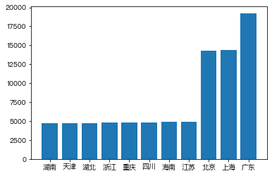
- 不同省份的订单数量
In [ ]:
df.groupby(by='省份').size().sort_values(ascending=False)Out[ ]:
省份
广东    80394
上海    61357
北京    58904
湖南    21520
江苏    21076
四川    20993
天津    20611
海南    20515
重庆    20239
浙江    19959
湖北    19859
dtype: int64- 不同省份的成交金额
In [ ]:
df.groupby(by='省份')['价格'].sum().sort_values(ascending=False)Out[ ]:
省份
广东    18307413.93
上海    13750759.16
北京    13079000.52
天津     4788590.02
湖南     4718300.37
江苏     4643938.88
四川     4641984.72
海南     4607828.72
浙江     4578588.07
湖北     4511041.06
重庆     4481221.61
Name: 价格, dtype: float64
用户消费行为分析
- 每个用户的总消费次数
In [ ]:
s1 = df.groupby(by='用户编号').size()
s1
Out[ ]:
用户编号
1515915625439951872     1
1515915625440038400     1
1515915625440099840     8
1515915625440121600     2
1515915625440881408    30
                       ..
1515915625514747648     4
1515915625514762240     1
1515915625514807296     2
1515915625514808064     1
1515915625514848512     2
Length: 83417, dtype: int64- 每个用户的总消费金额
In [ ]:
s2 = df.groupby(by='用户编号')['价格'].sum()
s2
Out[ ]:
用户编号
1515915625439951872      416.64
1515915625440038400       21.04
1515915625440099840     3843.57
1515915625440121600      182.83
1515915625440881408    19167.16
                         ...
1515915625514747648      703.38
1515915625514762240       11.55
1515915625514807296       20.09
1515915625514808064       39.10
1515915625514848512       67.09
Name: 价格, Length: 83417, dtype: float64- 探究用户消费次数和消费金额的关系
In [ ]:
plt.scatter(s1,s2)
plt.xlabel('用户消费次数')
plt.ylabel('用户消费金额')
Out[ ]:
Text(0, 0.5, '用户消费金额')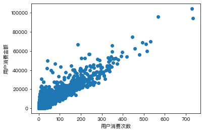
- 探究大部分用户消费次数的情况
In [ ]:
plt.hist(s1,bins=200)Out[ ]:
(array([6.5657e+04, 1.0875e+04, 2.8420e+03, 1.7350e+03, 7.8600e+02,
        2.7200e+02, 2.6200e+02, 1.4600e+02, 8.3000e+01, 6.0000e+01,
        4.8000e+01, 2.7000e+01, 4.0000e+01, 2.5000e+01, 2.2000e+01,
        2.4000e+01, 1.5000e+01, 1.8000e+01, 7.0000e+00, 1.2000e+01,
        1.4000e+01, 1.5000e+01, 1.2000e+01, 9.0000e+00, 1.1000e+01,
        1.5000e+01, 1.3000e+01, 1.2000e+01, 2.3000e+01, 5.0000e+00,
        1.2000e+01, 1.2000e+01, 1.1000e+01, 5.0000e+00, 1.3000e+01,
        7.0000e+00, 8.0000e+00, 8.0000e+00, 7.0000e+00, 8.0000e+00,
        6.0000e+00, 1.1000e+01, 7.0000e+00, 9.0000e+00, 3.0000e+00,
        1.1000e+01, 7.0000e+00, 5.0000e+00, 4.0000e+00, 1.2000e+01,
        1.0000e+01, 6.0000e+00, 2.0000e+00, 1.2000e+01, 8.0000e+00,
        7.0000e+00, 7.0000e+00, 5.0000e+00, 3.0000e+00, 4.0000e+00,
        2.0000e+00, 4.0000e+00, 5.0000e+00, 2.0000e+00, 2.0000e+00,
        8.0000e+00, 2.0000e+00, 4.0000e+00, 2.0000e+00, 1.0000e+00,
        4.0000e+00, 4.0000e+00, 2.0000e+00, 0.0000e+00, 2.0000e+00,
        4.0000e+00, 1.0000e+00, 2.0000e+00, 3.0000e+00, 5.0000e+00,
        3.0000e+00, 0.0000e+00, 1.0000e+00, 2.0000e+00, 2.0000e+00,
        0.0000e+00, 2.0000e+00, 0.0000e+00, 2.0000e+00, 2.0000e+00,
        3.0000e+00, 1.0000e+00, 2.0000e+00, 1.0000e+00, 1.0000e+00,
        2.0000e+00, 2.0000e+00, 1.0000e+00, 0.0000e+00, 0.0000e+00,
        1.0000e+00, 1.0000e+00, 0.0000e+00, 1.0000e+00, 0.0000e+00,
        0.0000e+00, 0.0000e+00, 1.0000e+00, 1.0000e+00, 0.0000e+00,
        0.0000e+00, 0.0000e+00, 0.0000e+00, 0.0000e+00, 1.0000e+00,
        0.0000e+00, 0.0000e+00, 0.0000e+00, 0.0000e+00, 0.0000e+00,
        0.0000e+00, 1.0000e+00, 0.0000e+00, 0.0000e+00, 1.0000e+00,
        0.0000e+00, 0.0000e+00, 0.0000e+00, 0.0000e+00, 0.0000e+00,
        1.0000e+00, 0.0000e+00, 0.0000e+00, 0.0000e+00, 1.0000e+00,
        0.0000e+00, 0.0000e+00, 0.0000e+00, 0.0000e+00, 1.0000e+00,
        1.0000e+00, 0.0000e+00, 0.0000e+00, 0.0000e+00, 1.0000e+00,
        0.0000e+00, 0.0000e+00, 0.0000e+00, 0.0000e+00, 0.0000e+00,
        0.0000e+00, 0.0000e+00, 0.0000e+00, 0.0000e+00, 1.0000e+00,
        0.0000e+00, 0.0000e+00, 0.0000e+00, 0.0000e+00, 0.0000e+00,
        0.0000e+00, 0.0000e+00, 0.0000e+00, 0.0000e+00, 0.0000e+00,
        0.0000e+00, 0.0000e+00, 0.0000e+00, 0.0000e+00, 0.0000e+00,
        0.0000e+00, 0.0000e+00, 0.0000e+00, 0.0000e+00, 0.0000e+00,
        0.0000e+00, 0.0000e+00, 0.0000e+00, 0.0000e+00, 0.0000e+00,
        0.0000e+00, 0.0000e+00, 0.0000e+00, 0.0000e+00, 0.0000e+00,
        0.0000e+00, 0.0000e+00, 0.0000e+00, 0.0000e+00, 0.0000e+00,
        0.0000e+00, 0.0000e+00, 0.0000e+00, 0.0000e+00, 0.0000e+00,
        0.0000e+00, 0.0000e+00, 0.0000e+00, 0.0000e+00, 2.0000e+00]),
 array([  1.  ,   4.66,   8.32,  11.98,  15.64,  19.3 ,  22.96,  26.62,
         30.28,  33.94,  37.6 ,  41.26,  44.92,  48.58,  52.24,  55.9 ,
         59.56,  63.22,  66.88,  70.54,  74.2 ,  77.86,  81.52,  85.18,
         88.84,  92.5 ,  96.16,  99.82, 103.48, 107.14, 110.8 , 114.46,
        118.12, 121.78, 125.44, 129.1 , 132.76, 136.42, 140.08, 143.74,
        147.4 , 151.06, 154.72, 158.38, 162.04, 165.7 , 169.36, 173.02,
        176.68, 180.34, 184.  , 187.66, 191.32, 194.98, 198.64, 202.3 ,
        205.96, 209.62, 213.28, 216.94, 220.6 , 224.26, 227.92, 231.58,
        235.24, 238.9 , 242.56, 246.22, 249.88, 253.54, 257.2 , 260.86,
        264.52, 268.18, 271.84, 275.5 , 279.16, 282.82, 286.48, 290.14,
        293.8 , 297.46, 301.12, 304.78, 308.44, 312.1 , 315.76, 319.42,
        323.08, 326.74, 330.4 , 334.06, 337.72, 341.38, 345.04, 348.7 ,
        352.36, 356.02, 359.68, 363.34, 367.  , 370.66, 374.32, 377.98,
        381.64, 385.3 , 388.96, 392.62, 396.28, 399.94, 403.6 , 407.26,
        410.92, 414.58, 418.24, 421.9 , 425.56, 429.22, 432.88, 436.54,
        440.2 , 443.86, 447.52, 451.18, 454.84, 458.5 , 462.16, 465.82,
        469.48, 473.14, 476.8 , 480.46, 484.12, 487.78, 491.44, 495.1 ,
        498.76, 502.42, 506.08, 509.74, 513.4 , 517.06, 520.72, 524.38,
        528.04, 531.7 , 535.36, 539.02, 542.68, 546.34, 550.  , 553.66,
        557.32, 560.98, 564.64, 568.3 , 571.96, 575.62, 579.28, 582.94,
        586.6 , 590.26, 593.92, 597.58, 601.24, 604.9 , 608.56, 612.22,
        615.88, 619.54, 623.2 , 626.86, 630.52, 634.18, 637.84, 641.5 ,
        645.16, 648.82, 652.48, 656.14, 659.8 , 663.46, 667.12, 670.78,
        674.44, 678.1 , 681.76, 685.42, 689.08, 692.74, 696.4 , 700.06,
        703.72, 707.38, 711.04, 714.7 , 718.36, 722.02, 725.68, 729.34,
        733.  ]),
 <BarContainer object of 200 artists>)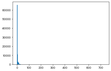
In [ ]:
s1.describe()Out[ ]:
count    83417.000000
mean         4.380726
std         15.136643
min          1.000000
25%          1.000000
50%          2.000000
75%          4.000000
max        733.000000
dtype: float64
In [ ]:
s2.describe()Out[ ]:
count     83417.000000
mean        984.315752
std        2510.050036
min           0.000000
25%         138.870000
50%         416.620000
75%        1018.470000
max      104501.240000
Name: 价格, dtype: float64- 新老用户的占比
- 消费次数为多次的(老用户),消费次数为1次(新用户)
In [ ]:
#消费多次(老用户),消费一次(新用户)
ret = df.groupby(by='用户编号')['下单日期'].agg(['min','max'])
ret
Out[ ]:
| min | max | |
|---|---|---|
| 用户编号 | ||
| 1515915625439951872 | 2020-07-09 | 2020-07-09 |
| 1515915625440038400 | 2020-09-22 | 2020-09-22 |
| 1515915625440099840 | 2020-05-21 | 2020-09-25 |
| 1515915625440121600 | 2020-05-16 | 2020-07-14 |
| 1515915625440881408 | 2020-05-20 | 2020-09-22 |
| ... | ... | ... |
| 1515915625514747648 | 2020-01-06 | 2020-09-21 |
| 1515915625514762240 | 2020-06-23 | 2020-06-23 |
| 1515915625514807296 | 2020-07-04 | 2020-07-04 |
| 1515915625514808064 | 2020-04-29 | 2020-04-29 |
| 1515915625514848512 | 2020-05-19 | 2020-05-19 |
83417 rows × 2 columns
In [ ]:
old_new_count = (ret['min'] == ret['max']).value_counts()
old_new_count
#True:新用户 False:老用户
Out[ ]:
True     45538
False    37879
dtype: int64
In [ ]:
plt.pie(old_new_count,labels=['新用户','老用户'],autopct='%.2f%%')Out[ ]:
([<matplotlib.patches.Wedge at 0x17aacc5b0>,
  <matplotlib.patches.Wedge at 0x17aacc400>],
 [Text(-0.15809694714931888, 1.0885795126227875, '新用户'),
  Text(0.15809694714931877, -1.0885795126227875, '老用户')],
 [Text(-0.08623469844508302, 0.5937706432487931, '54.59%'),
  Text(0.08623469844508296, -0.5937706432487931, '45.41%')])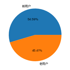
In [ ]:

 浙公网安备 33010602011771号