DS / ML Basic Notes
1 NumPy
1.1 Create Arrays
# Define in yourself
arr = np.array()

# 等差数列
arr = np.arange(size)
arr = np.linspace(start, end, step)

# 等比数列
arr = np.logspace(start, end, step)

# 生成随机数
arr = np.random.rand(size)
arr = np.random.randn(size)
arr = np.random.randint(low, high, size)

# 设置随机种子
np.random.seed(32)
1.2 Array Slicing
NumPy array vs. Python list
-
Similarity: NumPy array slicing is fundamentally similar to Python list slicing in many aspects, especially in the basic slicing syntax and logic.
-
Difference: NumPy array has Multi-Dimensional slicing and other advanced slicing(e.g. Boolean arrays).
syntax:
1-Dimensional Arrays: array[start:stop:step]
Multi-Dimensional Arrays: array[start1:stop1:step1, start2:stop2:step2, ...]
# 1-Dimensional Arrays
arr[1:5] # extract elements from index 1 to 4

# Multi-Dimensional Arrays
arr[2:5, 1:4] # extracts a subarray from rows 2 to 4 and columns 1 to 3

# Advanced slicing: Boolean arrays
arr[arr > 5]
1.3 Dimension
NumPy array vs. pd.Series vs. pd.DataFrame vs. torch.Tensor
# NumPy array, the shape is (rows, columns)
import numpy as np
array = np.array([[1, 2, 3], [4, 5, 6]])
print(array.shape) # (2, 3)
print(array.shape[0]) # 2


# pd.Series, the shape is (rows,)
import pandas as pd
series = pd.Series([1, 2, 3, 4, 5])
print(series.shape) # (5,)
print(series.shape[0]) # 5


# pd.DataFrame, the shape is (rows, columns)
import pandas as pd
data = {'Column1': [1, 2, 3, 4],
        'Column2': [5, 6, 7, 8],
        'Column3': [9, 10, 11, 12]}
df = pd.DataFrame(data)
print(df.shape) # (3, 4)
print(df.shape[0]) # 3


# torch.Tensor, the shape is (batch_size, num_channels, height, width)
import torch
tensor = torch.rand(10, 3, 64, 64)
print(tensor.shape)  # torch.Size([10, 3, 64, 64])
print(tensor.shape[0]) # 10
1.4 Statistics Function
import numpy as np

data = iris_df.iloc[:,0:4].values

np.mean(data)
np.mean(data, axis = 0) # along row direction
np.mean(data, axis = 1) # along column direction

np.average(data) # same as np.mean(data)
np.average(data, weights=(.1, .2, .4, .05, .05, .1, .1)) # calculate the weighted average of array

np.sum(data)
np.sum(data, axis = 0) # along row direction
np.sum(data, axis = 1) # along column direction

np.cumsum(data, axis = 0) # along row direction
np.cumprod(data, axis = 1) # along column direction

np.var(data) # variance
np.std(data) # standard deviation

np.max(data)
np.max(data, axis = 0) # along row direction
np.max(data, axis = 1) # along column direction

np.min(data)
np.min(data, axis = 0) # along row direction
np.min(data, axis = 1) # along column direction
2 Pandas
2.1 Series
<1> Covert
# Covert Pandas Series to NumPy array: return a NumPy array
df['Price'].values
# or
df['Price'].to_numpy()

# Covert Pandas Series to Python: return a list
df['Price'].to_list()
pd.Series([1, 2, 3]).to_list()
# Covert the date type from object to datatime, and extract the year
import pandas as pd

# if you use print(df.info()), the data type of Date is an object
data = {'Date': ['2021-01-01', '2022-02-15', '2023-03-20']}
df = pd.DataFrame(data)

# Convert the 'Date' column to datetime
df['Date'] = pd.to_datetime(df['Date'])

# Extract the year
df['Year'] = df['Date'].dt.year

print(df.info())
<2> Unique information
import pandas as pd
df = pd.DataFrame({'col1':[1,2,3,4],
				   'col2':[444,555,666,444],
				   'col3':['abc','def','ghi','xyz']})

df['col2'].unique() # array([444, 555, 666], dtype=int64)
df['col2'].value_counts()
df['col2'].apply(lambda x: x**2)
df.sort_values(by='col2') # inplace=False by default
2.2 DataFrame
<1> Checking the data property
The instantiated object can use the following method.
df = pd.read_csv('path')

# iterable objects
df.index
df.column

# shape and data type in each column
df.shape # return a tuple
df.dtypes # return a pd.Series

# take a first look
df.head()
df.info() # check data shape, types, null
df.describe() # statistics summary

# copy df to avoid in-place operations when plot and analyze
df.copy
<2> Slicing
pandas.DataFrame.iloc and pandas.DataFrame.loc
# Using index locator
df.iloc[1] # slicing row index = 1
df.iloc[:,0:3] # slicing all rows, and columns indexing from 0 to 2

# Using key locator
df.loc[1] # slicing row key = 1
df.loc['brand'] # slicing row key = 'brand'
Reference: pandas df.loc[] 与 df.iloc[] 详解及其区别 | CSDN
When you create your own dataset in PyTorch, and the column name is string (row index is number), you would like to use this code for get the data point.
# Create my dataset
from torch.utils.data import Dataset

class MyDataset(Dataset):

    def __init__(self) -> None:
        super().__init__()
        self.data = pd.read_csv("./ChnSentiCorp_htl_all.csv")
        self.data = self.data.dropna()

    def __getitem__(self, index):
		# 1st [] for row, 2nd [] for col, so then can get the data point.
        return self.data.iloc[index]["review"], self.data.iloc[index]["label"]

    def __len__(self):
        return len(self.data)


# Instantiation
dataset = MyDataset()
for i in range(5):
    print(dataset[i])

# output
'''
('距离川沙公路较近,但是公交指示不对,如果是"蔡陆线"的话,会非常麻烦.建议用别的路线.房间较为简单.', 1)
('商务大床房,房间很大,床有2M宽,整体感觉经济实惠不错!', 1)
('早餐太差,无论去多少人,那边也不加食品的。酒店应该重视一下这个问题了。房间本身很好。', 1)
('宾馆在小街道上,不大好找,但还好北京热心同胞很多~宾馆设施跟介绍的差不多,房间很小,确实挺小,但加上低价位因素,还是无超所值的;环境不错,就在小胡同内,安静整洁,暖气好足-_-||。。。呵还有一大优势就是从宾馆出发,步行不到十分钟就可以到梅兰芳故居等等,京味小胡同,北海距离好近呢。总之,不错。推荐给节约消费的自助游朋友~比较划算,附近特色小吃很多~', 1)
('CBD中心,周围没什么店铺,说5星有点勉强.不知道为什么卫生间没有电吹风', 1)
'''
Reference: 【手把手带你实战HuggingFace Transformers-入门篇】基础组件之Model | Bilibili
2.3 Missing values and duplicate values
<1> Check the number of missing values
pandas.Dataframe.isnull() and pandas.Dataframe.isna() are the same function.
df.isna().sum()
# or
df.isnull().sum()
<2> Check the proportion of missing values in each column
missing_proportion = df[df.columns].isnull().mean()
import pandas as pd
data = {
    'A': [1, None, 3, 4],
    'B': [None, 2, None, 4],
    'C': [1, 2, 3, None],
    'D': [None, None, None, None]
}
df = pd.DataFrame(data)

# Calculating the proportion of missing values in each column
missing_proportion = df[df.columns].isnull().mean()
print(missing_proportion)
<3> Handling missing values
np.mean(column_name) vs. DataFrame.column_name.mean()
# fill
data.loc[:,"Age"] = data.loc[:,"Age"].fillna(data.loc[:,"Age"].mean())
data.loc[:,"Age"] = data.loc[:,"Age"].fillna(data.loc[:,"Age"].median())
data.loc[:,"Age"] = data.loc[:,"Age"].fillna(data.loc[:,"Age"].mode())

# drop
data.dropna(axis=0,inplace=True) # delete the rows having np.nan
data.dropna(axis=1,inplace=True) # delete the columns having np.nan
<4> Check duplicate values
pandas.DataFrame.duplicated
df.duplicated().sum()
<5> Handling duplicate values
If there is duplicate rows, drop. pandas.DataFrame.drop_duplicates
df.drop_duplicates() # By default, it removes duplicate rows based on all columns.
df.drop_duplicates(subset=['brand', 'style']) # To remove duplicates on specific column(s), use subset.
2.4 Groupby and Pivot table
<1> Group by
syntax:
df.groupby(column_name)[column_name].mean()
df.groupby(column_name)[column_name].median()
df.groupby(column_name)[column_name].sum()
import pandas as pd

sales = pd.DataFrame({
    'type': ['A', 'B', 'A'],
    'weekly_sales': [200, 400, 150],
    'is_holiday': [False, False, True],
    'department': [1, 2, 3]
})

# Group by type; calc total weekly sales
sales_by_type = sales.groupby('type')['weekly_sales'].mean()
print(sales_by_type)

# Group by type and is_holiday; calc total weekly sales
sales_by_type_is_holiday = sales.groupby(["type", "is_holiday"])["weekly_sales"].sum()
print(sales_by_type_is_holiday)
<2> Pivot table
syntax:
df.pivot_table(values= ,index= ,columns= ,aggfunc= ,fill_value= ,margins= )
import numpy as np
import pandas as pd

sales = pd.DataFrame({
    'type': ['A', 'B', 'A'],
    'weekly_sales': [200, 400, 150],
    'is_holiday': [False, False, True],
    'department': [1, 2, 3]
})

# Pivot for mean weekly_sales for each store type
mean_sales_by_type = sales.pivot_table(values="weekly_sales", index = "type")

# Pivot for mean and median weekly_sales for each store type
mean_med_sales_by_type = sales.pivot_table(values='weekly_sales', index='type', aggfunc=[np.mean, np.median])

# Pivot for mean weekly_sales by store type and holiday
mean_sales_by_type_holiday = sales.pivot_table(values="weekly_sales", index="type", columns="is_holiday")

# Print the mean weekly_sales by department and type; fill missing values with 0s; sum all rows and cols
print(sales.pivot_table(values="weekly_sales", index="department", columns="type", fill_value=0, margins=True))
2.5 Merge, Join and Concat
syntax(concat)
pd.concat([df_1,df_2,...,df_n], axis =0)
syntax(merge)
pd.merge(df_left, df_right, on=[common_column] , how='inner')
syntax(join)
df_left.join(df_right)
# concat, which is along axis direction
import pandas as pd
df1 = pd.DataFrame({'A': ['A0', 'A1', 'A2', 'A3'],
                        'B': ['B0', 'B1', 'B2', 'B3'],
                        'C': ['C0', 'C1', 'C2', 'C3'],
                        'D': ['D0', 'D1', 'D2', 'D3']},
                        index=[0, 1, 2, 3])

df2 = pd.DataFrame({'A': ['A4', 'A5', 'A6', 'A7'],
                        'B': ['B4', 'B5', 'B6', 'B7'],
                        'C': ['C4', 'C5', 'C6', 'C7'],
                        'D': ['D4', 'D5', 'D6', 'D7']},
                         index=[4, 5, 6, 7])

df1_df2_axis0 = pd.concat([df1, df2])
df1_df2_axis1 = pd.concat([df1, df2], axis=1)

print(df1_df2_axis0)
print(df1_df2_axis1)
# merge, which logic is same as SQL join, can merge when there is either common column or no common column
import pandas as pd

left = pd.DataFrame({'key1': ['K0', 'K0', 'K1', 'K2'],
                     'key2': ['K0', 'K1', 'K0', 'K1'],
                     'A': ['A0', 'A1', 'A2', 'A3'],
                     'B': ['B0', 'B1', 'B2', 'B3']})

right = pd.DataFrame({'key1': ['K0', 'K1', 'K1', 'K2'],
                      'key2': ['K0', 'K0', 'K0', 'K0'],
                      'C': ['C0', 'C1', 'C2', 'C3'],
                      'D': ['D0', 'D1', 'D2', 'D3']})

df = pd.merge(left, right, how='inner', on='key1')
df1 = pd.merge(left, right, on=['key1', 'key2'])
df2 = pd.merge(left, right, how='right', on=['key1', 'key2'])
df3 = pd.merge(left, right, how='left', on=['key1', 'key2'])

print(df)
print(df1)
print(df2)
print(df3)
# join, which is the convenient way to merge tables when there is no common column name
import pandas as pd
left = pd.DataFrame({'A': ['A0', 'A1', 'A2'],
                     'B': ['B0', 'B1', 'B2']},
                      index=['K0', 'K1', 'K2'])

right = pd.DataFrame({'C': ['C0', 'C2', 'C3'],
                    'D': ['D0', 'D2', 'D3']},
                      index=['K0', 'K2', 'K3'])

left_right = left.join(right) # left join
left_right_outer = left.join(right, how='outer') # outer join

print(left_right)
print(left_right_outer)
2.6 Operations
filtered_df = df2[(df2['age'] == '[25:50)') & (df2['marital_stat']=='Widowed')]
filtered_df
2.7 I/O
import pandas as pd

# Add or Overwrite the header name
columns_name = ['age', 'class_of_worker', 'education', 'marital_stat', 'race', 'hispanic_origin', 'sex', 'member_of_a_labor_union', 'num_persons_worked_for_employer', 'family_members_under_18', 'country_of_birth_father', 'country_of_birth_mother', 'country_of_birth_self', 'citizenship', 'own_business_or_self_employed']
df2 = pd.read_csv('PartB/output/anonymized-k=4.txt', names=columns_name)
df2

# Save as csv
df2.to_csv('extract_dataframe.csv', index=False)
3 Matplotlib
Matplotlib.pyplot Official Document
import matplotlib.pyplot as plt

plt.figure()
plt.title()
plt.plot(x1= ,y1= ,color= ,marker= ,label=)
plt.plot(x2= ,y2= ,color= ,marker= ,label=)
plt.xlabel()
plt.ylabel()
plt.legend()
plt.show()
4 Seaborn
Seaborn Official Document

data: DataFrame
x: column_name
y: column_name
kind: axes-level choice
hue: add the categorical dimension to the plot
import seaborn as sns

sns.set_theme()

# displot commonly only uses x variable.
# hist can represent numerical variable distribution and categorical variable frequency.
sns.displot(data = penguins_df, x = '', hue = '', bins = 25)
# kde can represent density
sns.displot(data = penguins_df, x = '', kind = 'kde', hue = '')

# scatter can represent the relationship of two numerical variables
sns.relplot(data = penguins_df, x = '', y= '', kind = '')

# countplot is similar to the categorical part of histplot
# boxplot is commonly used to detect outliers
sns.catplot()

#
sns.lmplot()
5 Scikit-Learn
The data format expectations of Scikit-Learn
For features(i.e. independent variables), Scikit-Learn at least accept 2-D NumPy array or Pandas DataFrame.
For target(i.e. dependent variables), Scikit-Learn only accept 1-D NumPy array or Pandas DataFrame.
# Reshaping a single feature to a 2D array
X = df['feature'].values.reshape(-1,1)

# Flattening a target to a 1D array
y = df['target'].values.reshape(-1)
5.1 Metrics
- Metrics for Regression
- Metrics for Classification
- Metrics for Clustering
<1> Metrics for Regression
SSE(Sum of Squared Error) or RSS(Residual Sum of Squares), ranges from 0 to infinity
MAE(Mean Absolute Error), also called L1 regularization, ranges from 0 to infinity
scores can range from -∞ to 1, where a score of 1 indicates perfect prediction, 0 indicates that the model performs as well as a trivial baseline, and negative values indicate even worse performance. The bigger, the better.
from sklearn.metrics import mean_squared_error, mean_absolute_error, r2_score

# Create an Evaluate Function to give all metrics after model Training
def evaluate_model(y_true, y_pred):
    mae = mean_absolute_error(y_true, y_pred)
    mse = mean_squared_error(y_true, y_pred)
    rmse = np.sqrt(mean_squared_error(y_true, y_pred))
    r2_square = r2_score(y_true, y_pred)
    return mae, rmse, r2_square

# Evaluate Train and Test dataset
model_train_mae , model_train_rmse, model_train_r2 = evaluate_model(y_train, y_train_pred)
model_test_mae , model_test_rmse, model_test_r2 = evaluate_model(y_test, y_test_pred)
.score() in regression is a convenient method to calculate the R^2 score, no need to compute the y_pred at first.
# Instantiate
reg =

# Calculate the r^2 score
reg.score(X_test, y_test)

# Note: it is equivalent to the following method
y_pred = reg.predict(X_test)
r2_score = r2_score(y_test, y_pred)
<2> Metrics for Classification
from sklearn.metrics import coufusion_matrix, classification_report
from sklearn.metrics import accuracy_score
# confusion_matrix
cm = confusion_matrix(y_test, y_pred)
print("Confusion Matrix:")
print(cm)

ac = accuracy_score(y_test, y_pred)
print("\nAccuracy Score:")
print(ac)

# precision, recall, f1-score
cr = classification_report(y_test, y_pred)
print("\nClassification Report:")
print(cr)
.score() in classification is a convenient method to calculate the accuracy score, no need to compute the y_pred at first.
# Instantiate
clf =

# Calculate the accuracy score
clf.score(X_test, y_test)

# Note: it is equivalent to the following method
y_pred = clf.predict(X_test)
accuracy_score = accuracy_score(y_test, y_pred)
<3> Metrics for Clustering
from sklearn.cluster import KMeans
from sklearn.metrics import silhouette_score, davies_bouldin_score, calinski_harabasz_score
from sklearn.datasets import make_blobs

# Generate synthetic data for demonstration (you would use your own dataset here)
X, _ = make_blobs(n_samples=300, centers=4, cluster_std=0.60, random_state=0)

# Perform clustering using KMeans
kmeans = KMeans(n_clusters=4, random_state=0)
y_pred = kmeans.fit_predict(X)

# Evaluate the clustering
silhouette_avg = silhouette_score(X, y_pred)
davies_bouldin = davies_bouldin_score(X, y_pred)
calinski_harabasz = calinski_harabasz_score(X, y_pred)

print("Silhouette Score: ", silhouette_avg)
print("Davies-Bouldin Index: ", davies_bouldin)
print("Calinski-Harabasz Index: ", calinski_harabasz)
5.2 - Cross Validation & Hyperparameter Tuning
<1> libararies
from sklearn.model_selection import train_test_split # split the full dataset into training and testing
from sklearn.model_selection import KFold # More options for cv argument. in cross validation, like fixed the random_state
from sklearn.model_selection import cross_val_score # Cross Validation
from sklearn.model_selection import GridSearchCV # Grid Search(for Hyperparameter Tuning) + Cross Validation
from sklearn.model_selection import RandomizedSearchCV # an alternative approach
<2> Example for cross_val_score
scoring = 'neg_mean_squared_error' or 'neg_mean_absolute_error' or 'r2', default = 'r2'
scores = cross_val_score(model, X, y, cv=5, scoring='neg_mean_squared_error') # Use 'neg_mean_squared_error' as scoring parameter
mse_scores = -scores # Since the scores are negative, you need to convert them to positive values to interpret them as MSE. This is a (cv,) shape vector.
average_mse = mse_scores.mean() # Optionally, you can calculate the average MSE across all folds for an overall performance metric.
<3> Example for GridSearchCV
from sklearn.model_selection import GridSearchCV

kf = KFold(n_splits=5, shuffle=True, random_state=42)

param_grid = {"alpha": np.arange(0.0001, 1, 10),
			  "solver": ["sag","lsqr"]}

ridge = Ridge()
ridge_cv = GridSearchCV(ridge, param_grid, cv=kf)
ridge_cv.fit(X_train, y_train)
print(ridge_cv.best_params_, ridge_cv.best_score_)
{'alpha': 0.0001, 'solver': 'sag'}
0.7529912278705785
Here are the Hyperparameters in Machine Learning model.
# Lasso Regression
from sklearn.linear_model import Lasso

model = Lasso()
param_grid = {
    'alpha': [0.001, 0.01, 0.1, 1, 10, 100],
    'max_iter': [1000, 5000, 10000],
    'tol': [0.0001, 0.001, 0.01]
}


# Ridge Regression
from sklearn.linear_model import Ridge

model = Ridge()
param_grid = {
    'alpha': [0.001, 0.01, 0.1, 1, 10, 100],
    'solver': ['auto', 'svd', 'cholesky', 'lsqr', 'sparse_cg', 'sag', 'saga']
}


# Logistic Regression
from sklearn.linear_model import LogisticRegression

model = LogisticRegression()
param_grid = {
    'C': [0.001, 0.01, 0.1, 1, 10, 100],
    'penalty': ['l1', 'l2'],
    'max_iter': [100, 200, 300],
    'solver': ['newton-cg', 'lbfgs', 'liblinear', 'sag', 'saga']
}

#  Support Vector Machine (SVM)
from sklearn.svm import SVC

model = SVC()
param_grid = {
    'C': [0.1, 1, 10, 100],
    'kernel': ['linear', 'rbf', 'poly'],
    'gamma': ['scale', 'auto']
}


# Decision Tree
from sklearn.tree import DecisionTreeClassifier

model = DecisionTreeClassifier()
param_grid = {
    'max_depth': [None, 10, 20, 30],
    'min_samples_split': [2, 5, 10],
    'min_samples_leaf': [1, 2, 4]
}


# Random Forest
from sklearn.ensemble import RandomForestClassifier
model = RandomForestClassifier()

param_grid = {
    'n_estimators': [10, 50, 100, 200],
    'max_depth': [None, 10, 20, 30],
    'min_samples_split': [2, 5, 10],
    'min_samples_leaf': [1, 2, 4],
    'bootstrap': [True, False]
}


# XGBoost
from xgboost import XGBRegressor
model = XGBRegressor()

param_grid = {
    'learning_rate': [0.01, 0.1, 0.2, 0.3],
    'max_depth': [3, 4, 5, 6],
    'n_estimators': [50, 100, 200],
    'subsample': [0.5, 0.7, 1.0],
    'colsample_bytree': [0.5, 0.7, 1.0]
}
5.3 Handling missing values
Using Pandas is simpler: Pandas missing values
sklearn.impute.SimpleImputer
class sklearn.impute.SimpleImputer(missing_values=nan, strategy='mean', fill_value=None, copy=True)
variable = Class.method_1.method_2.method_n
from sklearn.impute import SimpleImputer

# Instantiate an object
imp_mean = SimpleImputer()
imp_median = SimpleImputer(strategy='median')
imp_mode = SimpleImputer(strategy='most_frequent')
imp_constant = SimpleImputer(strategy='constant',fill_value=0)
🌰 For instance
### Step by step code
# fill with mode value in the 'Embarked' field
Embarked = data.loc[:,'Embarked'].values.reshape(-1,1) # the feature matrix must be 2D
imp_mode = SimpleImputer(strategy='most_frequent') # instantiate an object
data.loc[:,'Embarked'] = imp_mode.fit_transform(Embarked)

### Clean code
# fill with mode value in the 'Embarked' field
data.loc[:,'Embarked'] = SimpleImputer(strategy='most_frequent').fit_transform(data.loc[:,'Embarked'].values.reshape(-1,1))
5.4 Categorical variables
- One Hot
- Scikit-Learn:
OneHotEncoder() - Pandas:
get_dummies()
- Scikit-Learn:
- Multi-class Label
LabelEncoder()
categorical_features = [feature for feature in df.columns if df[feature].dtype == 'O']
df = pd.get_dummies(df, columns=categorical_features,dtype=int)
label_encoder = LabelEncoder()
for feature in categorical_features:
    df_train[feature] = label_encoder.fit_transform(df_train[feature])
from sklearn.preprocessing import OneHotEncoder()
5.5 Data scaling
Normalization数据归一化,归一化后服从正态分布,feature_range默认为[0,1],默认数据压缩到[0,1]的范围
公式如下:
from sklearn.preprocessing import MinMaxScaler
Standardization(Z-score nomalization)数据标准化,数据会服从为均值为0,方差为1的正态分布(标准正态分布)
from sklearn.preprocessing import StandardScaler
# Create Column Transformer with 3 types of transformers
num_features = X.select_dtypes(exclude="object").columns
cat_features = X.select_dtypes(include="object").columns

from sklearn.preprocessing import OneHotEncoder, StandardScaler
from sklearn.compose import ColumnTransformer

numeric_transformer = StandardScaler()
oh_transformer = OneHotEncoder()

preprocessor = ColumnTransformer(
    [
        ("OneHotEncoder", oh_transformer, cat_features),
         ("StandardScaler", numeric_transformer, num_features),
    ]
)

# train and export results
X = preprocessor.fit_transform(X)
5.6 Imbalanced data
6 Pipeline
6.1 Data Preprocessing
Data Preprocessing means converting raw data to useful data.
-
Feature Engineering (Takes 30% of Project Time)
- EDA
- Analyze how many numerical features are present using histogram, pdf with seaborn, matplotlib.
- Analyze how many categorical features are present. Is multiple categories present for each feature?
- Missing Values (Visualize all these graphs)
- Outliers - Boxplot
- Cleaning
- Handling the Missing Values
- Mean/Median/Mode
- Handling Imbalanced dataset
- Treating the Outliers
- Scaling down the data - Standardization, Normalization
- Converting the categorical features into numerical features
- EDA
-
Feature Selection
- Correlation
- KNeighbors
- ChiSquare
- Genetic Algorithm
- Feature Importance - Extra Tree Classifiers
-
Model Creation
-
Hyperparameter Tuning
-
Model Deployment
-
Incremental Learning
6.2 Model Selection
Supervised Learning
- Linear Model
- Linear Regression
- Logistic Regression
- Genelized Linear Models
- Support Vector Machine, SVM
- Generative Learning
- Naive Bayes
- Tree-based and Ensemble Methods
- CART: Decision Tree, Regression Tree
- Random forest
- Boosting: Adaptive Boosting(e.g. Adaboost), Gradient Boosting(e.g. XGboost, LightGBM)
- k-nearest neighbors, KNN
Unsupervised Learning
- Clustering
- kmeans
- Dimension Reduction
- PCA
- PCA
6.3 Metrics
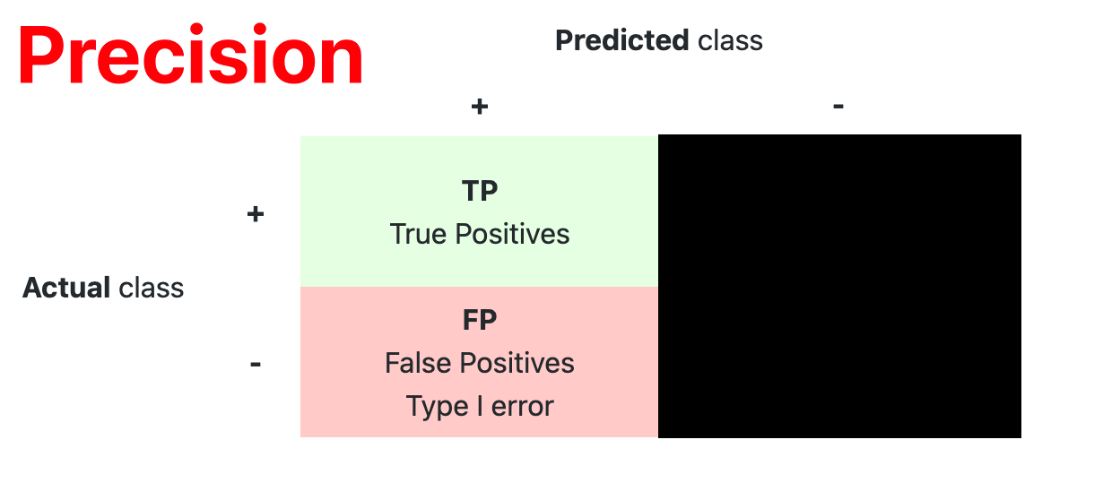
- Confusion Matrix
The confusion matrix is used to have a more complete picture when assessing the performance of a model. It is defined as follows:
- Main Metric
The following metrics are commonly used to assess the performance of classification models:| Metric | Formula | Interpretation |
|---|---|---|
| Accuracy | Overall performance of model | |
| Precision | How accurate the positive predictions are | |
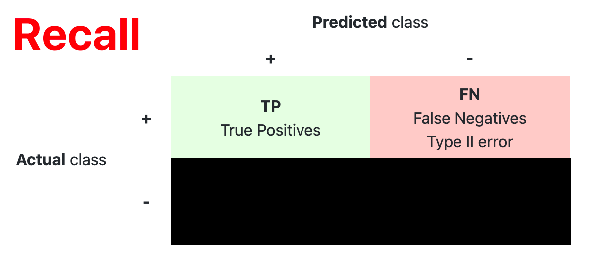
| Recall (Sensitivity) | Coverage of actual positive sample | |
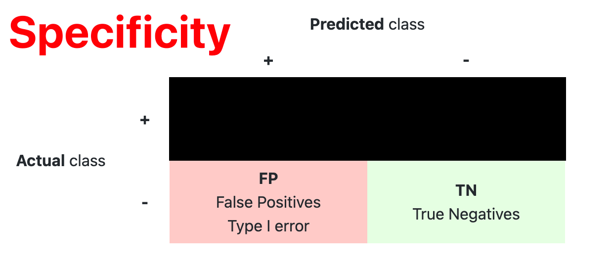
| Specificity | Coverage of actual negative sample | |
| F-score | Hybrid metric useful for unbalanced classes | |
| F-score | F-1 score generalized form ( = 1) |
- The importance of , need to be high, < 1 (spam or not, FP may miss something important)
- The importance of , need to be high, > 1 (cancer or not, FN may miss cancer symptoms)
- The importance of , = 1
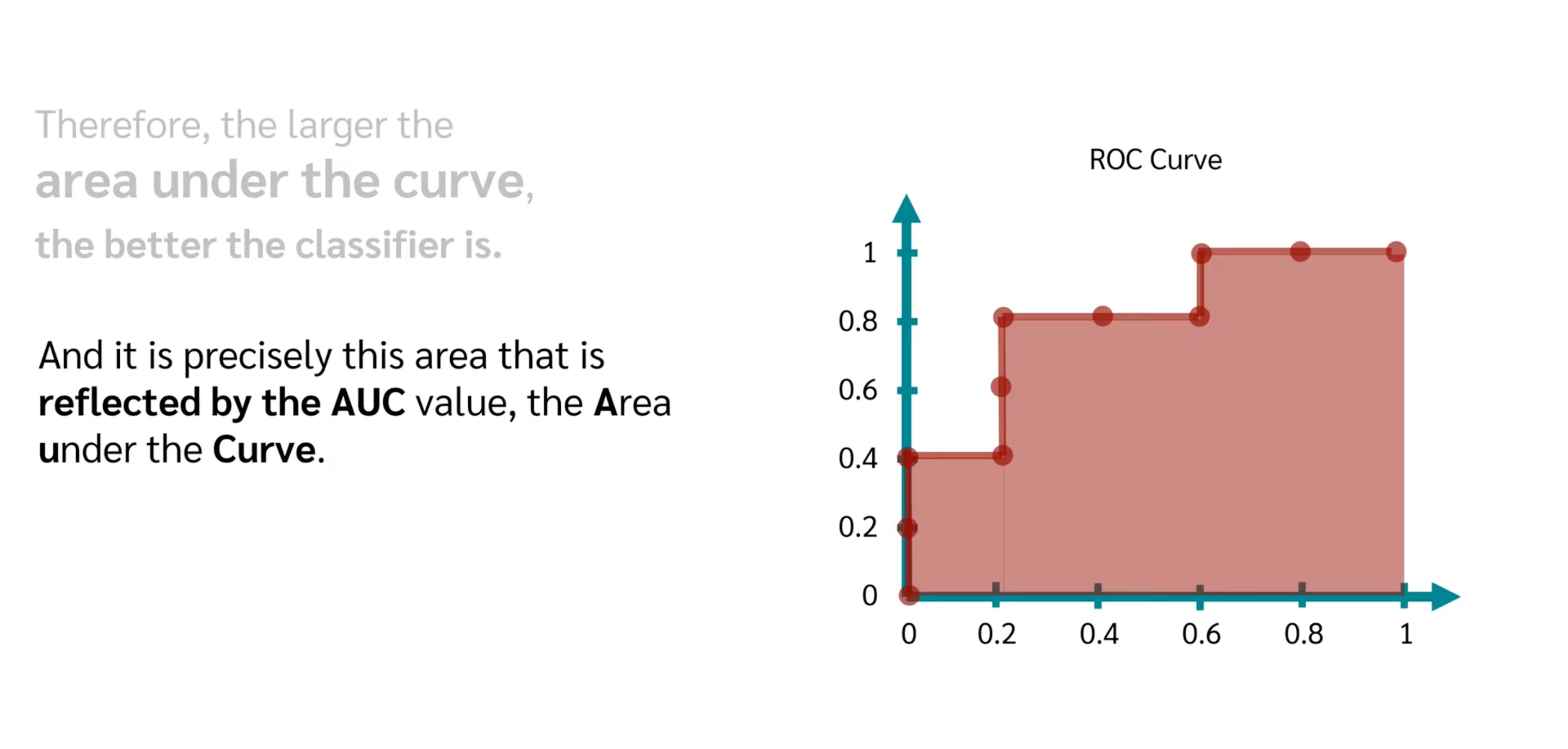
- ROC
| Metric | Formula | Interpretation |
|---|---|---|
| True Positive Rate(TPR) | Recall(Sensitivity) | |
| False Positive Rate(FPR) | 1-Specificity |
- x-axis is TPR, y-axis is FPR.
- The threshold changes from 0 to m, meanwhile the coordinate changes from top-right to bottom-left.The coordinate is (The quantity of TP, The quantity of FP) under the threshold
- choose the most left-top one.
- y = x curve commonly drawed a dummy line is the random selection case, without model.
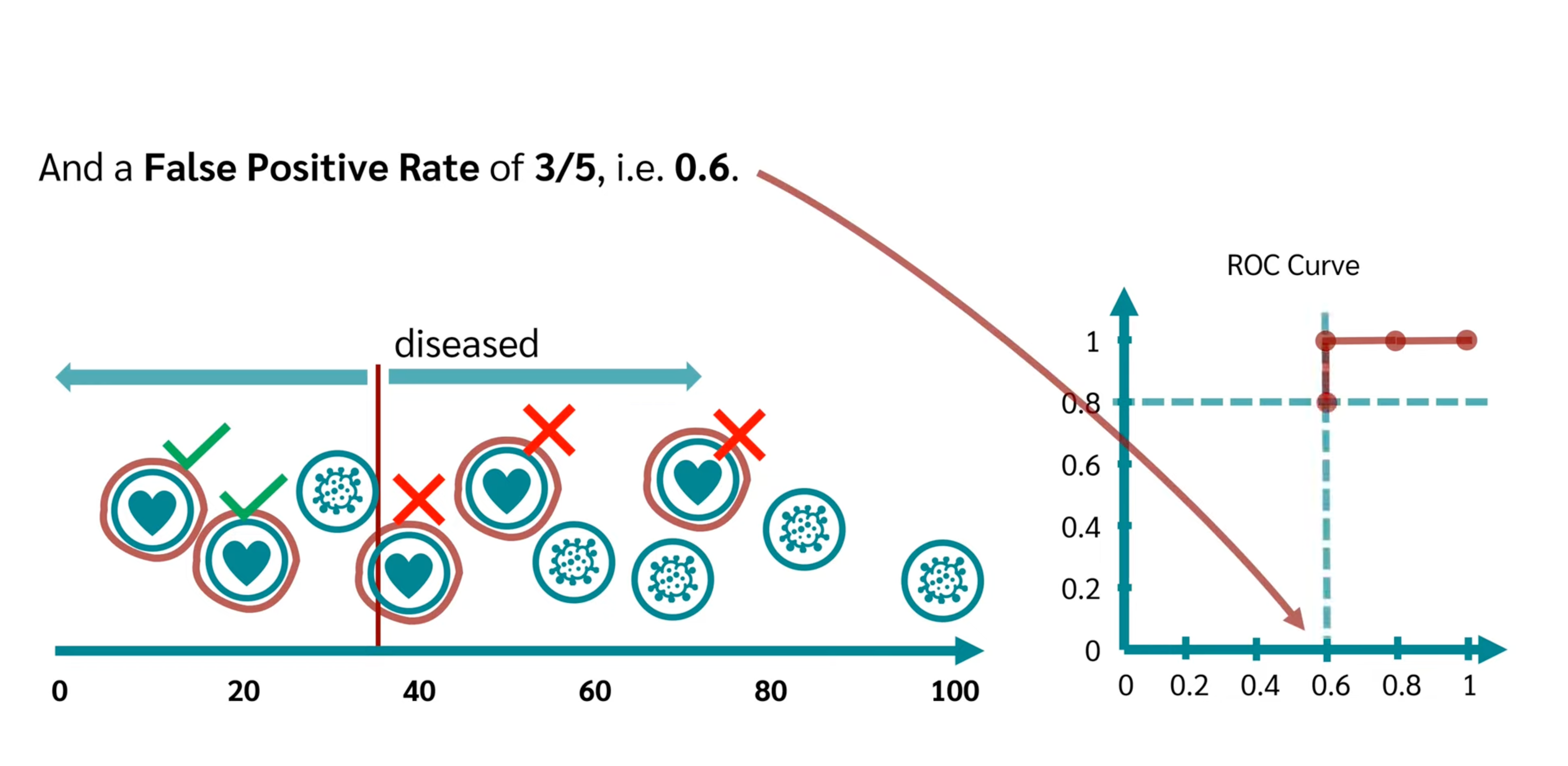
- AUC
The closer to 1, the better model score and threshold selection.
ROC and AUC, Clearly Explained!
ROC curve and AUC value Explanation
For more details:
Tutorial 34- Performance Metrics For Classification Problem In Machine Learning- Part1
Tutorial 41-Performance Metrics(ROC,AUC Curve) For Classification Problem In Machine Learning Part 2
Performance Metrics On MultiClass Classification Problems
Machine Learning-Bias And Variance In Depth Intuition| Overfitting Underfitting


【推荐】编程新体验,更懂你的AI,立即体验豆包MarsCode编程助手
【推荐】凌霞软件回馈社区,博客园 & 1Panel & Halo 联合会员上线
【推荐】抖音旗下AI助手豆包,你的智能百科全书,全免费不限次数
【推荐】博客园社区专享云产品让利特惠,阿里云新客6.5折上折
【推荐】轻量又高性能的 SSH 工具 IShell:AI 加持,快人一步
· DeepSeek “源神”启动!「GitHub 热点速览」
· 微软正式发布.NET 10 Preview 1:开启下一代开发框架新篇章
· 我与微信审核的“相爱相杀”看个人小程序副业
· C# 集成 DeepSeek 模型实现 AI 私有化(本地部署与 API 调用教程)
· spring官宣接入deepseek,真的太香了~