TF - CNN

目录

• 卷积网络
  • 卷积层
  • 第二个卷积层
  • 全连接层
• 求解

---

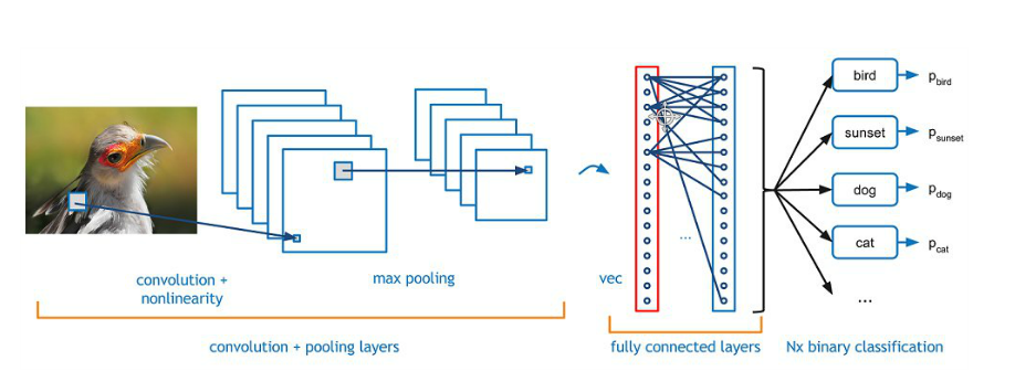
卷积网络

import tensorflow as tf
import random
import numpy as np
import matplotlib.pyplot as plt
import datetime
%matplotlib inline

from tensorflow.examples.tutorials.mnist import input_data
mnist = input_data.read_data_sets("data/", one_hot=True)

Extracting data/train-images-idx3-ubyte.gz
Extracting data/train-labels-idx1-ubyte.gz
Extracting data/t10k-images-idx3-ubyte.gz
Extracting data/t10k-labels-idx1-ubyte.gz

---

tf.reset_default_graph() 
sess = tf.InteractiveSession()
x = tf.placeholder("float", shape = [None, 28,28,1]) #shape in CNNs is always None x height x width x color channels
y_ = tf.placeholder("float", shape = [None, 10]) #shape is always None x number of classes

---

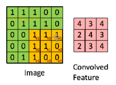
卷积层

W_conv1 = tf.Variable(tf.truncated_normal([5, 5, 1, 32], stddev=0.1))#shape is filter x filter x input channels x output channels
b_conv1 = tf.Variable(tf.constant(.1, shape = [32])) #shape of the bias just has to match output channels of the filter

---

h_conv1 = tf.nn.conv2d(input=x, filter=W_conv1, strides=[1, 1, 1, 1], padding='SAME') + b_conv1
h_conv1 = tf.nn.relu(h_conv1)
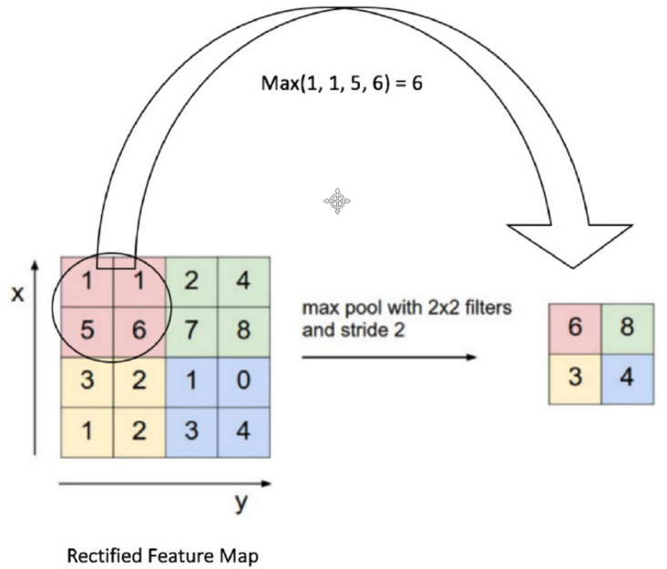
h_pool1 = tf.nn.max_pool(h_conv1, ksize=[1, 2, 2, 1], strides=[1, 2, 2, 1], padding='SAME')

def conv2d(x, W):
    return tf.nn.conv2d(input=x, filter=W, strides=[1, 1, 1, 1], padding='SAME')

def max_pool_2x2(x):
    return tf.nn.max_pool(x, ksize=[1, 2, 2, 1], strides=[1, 2, 2, 1], padding='SAME')

第二个卷积层

# Second Conv and Pool Layers  第二个卷积层
W_conv2 = tf.Variable(tf.truncated_normal([5, 5, 32, 64], stddev=0.1)) # 32-第一次卷积后得到32个特征图 
b_conv2 = tf.Variable(tf.constant(.1, shape = [64]))
h_conv2 = tf.nn.relu(conv2d(h_pool1, W_conv2) + b_conv2)
h_pool2 = max_pool_2x2(h_conv2)

# 卷积层只是进行特征提取，最终还是需要全连接层 来利用特征

全连接层

# First Fully Connected Layer 第一个全连接层
W_fc1 = tf.Variable(tf.truncated_normal([7 * 7 * 64, 1024], stddev=0.1)) 
# 7 - 28经过两次 relu 变成 7；有64个图；将这些特征转换为 1024 维特征

b_fc1 = tf.Variable(tf.constant(.1, shape = [1024])) # 输出 1024，所以b也是1024

h_pool2_flat = tf.reshape(h_pool2, [-1, 7*7*64]) # 将上述特征矩阵拉长为一条，来执行全连接任务

h_fc1 = tf.nn.relu(tf.matmul(h_pool2_flat, W_fc1) + b_fc1) 

# Dropout Layer 
keep_prob = tf.placeholder("float")
h_fc1_drop = tf.nn.dropout(h_fc1, keep_prob)  # 保留率

# Second Fully Connected Layer 第二个全连接层
W_fc2 = tf.Variable(tf.truncated_normal([1024, 10], stddev=0.1)) # 将 1024 个特征映射为 10 个分类。
b_fc2 = tf.Variable(tf.constant(.1, shape = [10]))

# Final Layer
y = tf.matmul(h_fc1_drop, W_fc2) + b_fc2

求解

crossEntropyLoss = tf.reduce_mean(tf.nn.softmax_cross_entropy_with_logits(labels = y_, logits = y)) # 损失函数
trainStep = tf.train.AdamOptimizer().minimize(crossEntropyLoss)
# 这里使用 Adam, Adam 相比 梯度下降(学习率不变)，原理相似，会自适应调整学习率，学习率一次比一次小，更常用。

correct_prediction = tf.equal(tf.argmax(y,1), tf.argmax(y_,1))
accuracy = tf.reduce_mean(tf.cast(correct_prediction, "float"))

sess.run(tf.global_variables_initializer())

batchSize = 50
for i in range(1000):
    batch = mnist.train.next_batch(batchSize)
    trainingInputs = batch[0].reshape([batchSize,28,28,1])
    trainingLabels = batch[1]
    if i%100 == 0:
        trainAccuracy = accuracy.eval(session=sess, feed_dict={x:trainingInputs, y_: trainingLabels, keep_prob: 1.0})
        print ("step %d, training accuracy %g"%(i, trainAccuracy))
    trainStep.run(session=sess, feed_dict={x: trainingInputs, y_: trainingLabels, keep_prob: 0.5})

step 0, training accuracy 0.14
step 100, training accuracy 0.94
step 200, training accuracy 0.96
step 300, training accuracy 0.98
step 400, training accuracy 0.96
step 500, training accuracy 1
step 600, training accuracy 0.98
step 700, training accuracy 0.98
step 800, training accuracy 1
step 900, training accuracy 0.98