详细推导线性回归

详细推导线性回归

关键词：线性回归; linear Regression.

绪论

根据李航的归纳，机器学习模型有三要素，分别是：模型、策略和算法。为了简单好记，本文认为，在线性回归问题中，模型、策略和算法可以做如下简记：

模型 = 模型
策略 = 损失函数 + 优化目标
算法 = 解析解/数值计算方法 = 梯度下降方法

数学推导

建立模型

假设输出变量 \(\hat{y}\) 与输入变量 \(x_1\) 和 \(x_2\) 的关系为：

\[\hat{y} = \hat{w_1} x_1 + \hat{w_2} x_2 + \hat{b} \]

建立上述模型的目的是为要拟合如下线性关系：

\[y = w_1 x_1 + w_2 x_2 + b \]

设定策略

设模型的损失函数为平方损失：

\[L(\hat{w_1}, \hat{w_2}, \hat{b}) = \frac{1}{n} \sum_{i=1}^{n} L^{(i)}(\hat{w_1}, \hat{w_2}, \hat{b}) = \frac{1}{n} \sum_{i=1}^{n} \frac{1}{2}(\hat{y}^{(i)} - y^{(i)})^2 \]

目标函数为：

\[w_1^*, w_2^*, b^* = \mathop{\arg\min}_{w_1, w_2, b} \ L(\hat{w_1}, \hat{w_2}, \hat{b}) \]

选择优化方法

梯度下降

采用梯度下降方法更新参数的公式如下：

\[\hat{w_1} = \hat{w_1} - \eta\frac{\partial{L}}{\partial{\hat{w_1}}} \\ \hat{w_2} = \hat{w_2} - \eta\frac{\partial{L}}{\partial{\hat{w_2}}} \\ \hat{b} = \hat{b} - \eta\frac{\partial{L}}{\partial{\hat{b}}} \]

为了方便理解，下面借助于复合函数求导法则将 \(\frac{\partial L}{\partial w_1}\) ， \(\frac{\partial L}{\partial w_1}\) 和 \(\frac{\partial L}{\partial w_1}\) 分别展开：

\[\begin{align} \frac{\partial L}{\partial \hat{w_1}} & = \frac{\partial \frac{1}{2} (\hat{y}-y)^2}{\partial \hat{y}} \cdot \frac{\partial \hat{y}}{\partial \hat{w_1}} \\ & = \frac{1}{2} \cdot 2 \cdot (\hat{y} - y) \cdot x_1 \\ & = (\hat{y} - y) \cdot x_1 \\ \frac{\partial L}{\partial \hat{w_2}} &= (\hat{y} - y) \cdot x_2 \\ \frac{\partial L}{\partial \hat{b}} &= \hat{y} - y \end{align} \]

模型参数在整个数据集上的更新公式如下：

\[\hat{w_1} = \hat{w_1} - \frac{\eta}{n}\sum_{i\in{n}}(\hat{y}^{(i)} - y^{(i)})x_{1}^{(i)} \\ \hat{w_2} = \hat{w_2} - \frac{\eta}{n}\sum_{i\in{n}}(\hat{y}^{(i)} - y^{(i)})x_{2}^{(i)} \\ \hat{b} = \hat{b} - \frac{\eta}{n}\sum_{i\in{n}}(\hat{y}^{(i)} - y^{(i)}) \]

小批量随机梯度下降

本文选用小批量随机梯度下降（mini-batch Stochastic Gradient Descend）方法来优化模型，设每次取得的批量大小为 \(|\mathcal{B}|\)，则模型的近似平均损失如下：

\[L = \frac{1}{|\mathcal{B}|} \sum_{i=1}^{|\mathcal{B}|} \frac{1}{2}(\hat{y}^{(i)} - y^{(i)})^2 \]

采用了小批量随机梯度下降的 \(\frac{\partial L}{\partial w_1}\) ， \(\frac{\partial L}{\partial w_1}\) 和 \(\frac{\partial L}{\partial w_1}\) 分别展开：

\[\begin{align} \frac{\partial L}{\partial \hat{w_1}} & = \frac{\partial \frac{1}{|\mathcal{B}|} \sum_{i=1}^{|\mathcal{B}|} \frac{1}{2} (\hat{y}^{(i)}-y^{(i)})^2}{\partial \hat{w_1}} \\ & = \frac{1}{\mathcal{|B|}} \sum_{i=1}^{\mathcal{|B|}} (\hat{y}^{(i)} - y^{(i)}) x_{1}^{(i)} \\ \frac{\partial L}{\partial \hat{w_2}} & = \frac{1}{\mathcal{|B|}} \sum_{i=1}^{\mathcal{|B|}} (\hat{y}^{(i)} - y^{(i)}) x_{2}^{(i)} \\ \frac{\partial L}{\partial \hat{b}} & = \frac{1}{\mathcal{|B|}} \sum_{i=1}^{\mathcal{|B|}} (\hat{y}^{(i)} - y^{(i)}) \\ \end{align} \]

模型各个参数的更新方法如下：

\[\hat{w_1} = \hat{w_1} - \frac{\eta}{\mathcal{|B|}} \sum_{i\in{\mathcal{B}}} (\hat{y}^{(i)} - y^{(i)}) x_{1}^{(i)} \\ \hat{w_2} = \hat{w_2} - \frac{\eta}{\mathcal{|B|}} \sum_{i\in{\mathcal{B}}} (\hat{y}^{(i)} - y^{(i)}) x_{2}^{(i)} \\ \hat{b} = \hat{b} - \frac{\eta}{\mathcal{|B|}} \sum_{i\in{\mathcal{B}}} (\hat{y}^{(i)} - y^{(i)}) \]

编码实现

基于小批量梯度下降的线性回归：使用 Python3 实现

# coding=utf-8

import numpy as np
from matplotlib import pyplot as plt


def generate_data(w, b, sample_num):
    feature_num = len(w)
    w = np.array(w).reshape(-1, 1)
    x = np.random.random(sample_num * feature_num).reshape(sample_num, feature_num)
    varepsilon = np.random.normal(size=(sample_num, 1))
    y = np.matmul(x, w) + b + varepsilon
    return x, y


class LinearRegression:
    def __init__(self, lr=0.001):
        self.eta = lr

    def fit(self, x, y, epochs=30, batch_size=32):
        losses = list()
        sample_num, feature_num = x.shape
        self.w, self.b = np.random.normal(size=(feature_num, 1)), np.random.random()
        batch_num = sample_num / batch_size if sample_num % batch_size == 0 else int(sample_num / batch_size) + 1
        for epoch in range(epochs):
            for batch in range(batch_num):
                x_batch = x[batch*batch_size:(batch+1)*batch_size, :]
                y_batch = y[batch*batch_size:(batch+1)*batch_size]
                y_batch_pred = self.predict(x_batch)
                error = y_batch_pred - y_batch
                average_error = np.average(error)
                self.b = self.b - self.eta * average_error
                for i in range(feature_num):
                    gradient = error * x[:, i]
                    average_gradient = np.average(gradient)
                    self.w[i] = self.w[i] - self.eta * average_gradient
            y_pred = self.predict(x)
            error = y_pred - y
            loss = np.average(error * error / 2)
            print("[Epoch]%d [Loss]%f [w1]%.2f [w2]%.2f [b]%.2f" % (epoch, loss, self.w[0], self.w[1], self.b))
            losses.append(loss)
        return losses

    def predict(self, x):
        left = np.matmul(x, self.w)
        y = left + b
        return y


if __name__ == '__main__':
    sample_num = 1000
    w = [2.5, 1.3]
    b = 1.8
    x, y = generate_data(w, b, sample_num)

    lr = LinearRegression(lr=0.001)
    loss = lr.fit(x, y, epochs=300)
    plt.plot(loss)
    plt.show()

实验

本文的实验数据，是按照如下方法生成的：

\[y = xw + b + \varepsilon \]

其中，\(W=[2.5, 1.3]^{\mathrm{ T }}\) ， \(b=1.8\) ， \(\varepsilon \sim \mathcal{N(1, 0)}\) ，生成的数据样本数为 1000。

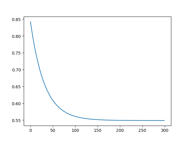
实验结果：

[Epoch]299 [Loss]0.548715 [w1]1.87 [w2]1.88 [b]2.40

损失图像：

结论

在本文中，我们有如下贡献：

1. 推导了线性回归算法；
2. 推导了小批量随机梯度下降；
3. 实现了基于小批量随机梯度下降的线性回归算法。

通过实验，我们有如下结论：

1. 小批量随机梯度下降对参数的更新次数远远大于梯度下降；
2. 直觉上，在同样的超参数设置下，小批量随机梯度下降可以比梯度更好地优化模型，得到更低的损失。