
DeepLabV3+网络模型与源码解读
源码链接:
链接:https://pan.baidu.com/s/1GkUM9WiGpzUHuFgBe1t2rA
提取码:57zr
or
https://github.com/VainF/DeepLabV3Plus-Pytorch
以上两个连接是一样的,只不过百度盘中的包含voc数据。
环境安装:
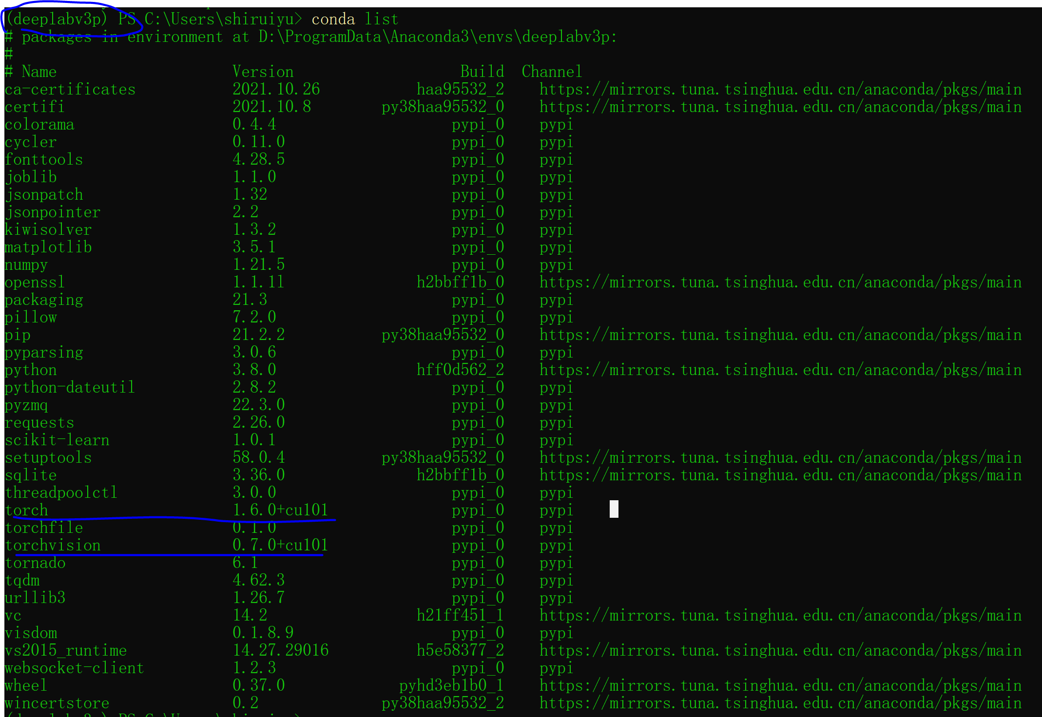
先装pytorch&torchvision,再安装requirments.txt其他依赖
报错处理:
# error:raise ValueError("cannot allocate more than 256 colors") from e
# solution:将batch_size由16改为4
源码中,main.py既可以用于训练,也可以用于测试,命令行参数如下:
 1 """
 2 训练:
 3 --model deeplabv3plus_mobilenet
 4 --gpu_id 0
 5 --year 2012_aug
 6 --crop_val
 7 --lr 0.01
 8 --crop_size 513
 9 --batch_size 4
10 --output_stride 16
11 测试:
12 --model deeplabv3plus_mobilenet
13 --gpu_id 0 --year 2012_aug
14 --crop_val
15 --lr 0.01
16 --crop_size 513
17 --batch_size 16
18 --output_stride 16
19 --ckpt checkpoints/best_deeplabv3plus_mobilenet_voc_os16.pth
20 --test_only
21 --save_val_results
22 """
- 一、网络概述
- 二、BackBone
- 三、Neck:ASPP
- 3.1 空洞卷积
- 3.2 感受野
- 3.3 SPP
- 3.4 ASPP
- 四、Head:DeepLabHead
- 五、性能评估
- 六、模型部署
一、网络概述
输入图像为:N*3*513*513,输出特征图为:N*C*513*513(N表示batch_size,C表示分类别数)。网络主要包含两部分:
EnCoder:一个BackBone和ASPP
Decoder:特征融合,进一步提取。
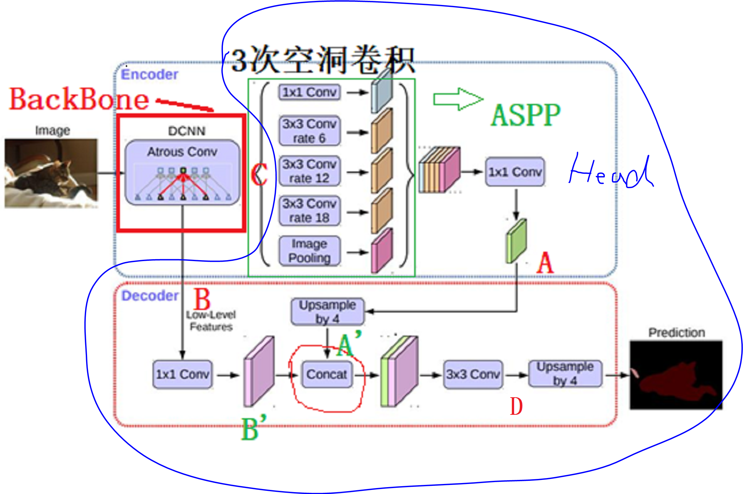
对于BackBone可选的有:resnet50、restnet101,mobilenet(v2版本,显然最快),代码会自动下载与训练模型,默认存储路径:C:\Users\shiruiyu\.cache\torch\hub\checkpoints 。如下图,BackBone即:DCNN(以restnet50为例),输出5组特征:
layer1、layer2、layer3、layer4、layer5;layer1表示low-Level Features,记为B,layer5表示高层特征,记为C。
将C输入到ASPP中得到A,然后上采样得到A‘,将B进一步处理得到B’,然后将A‘、B’叠加......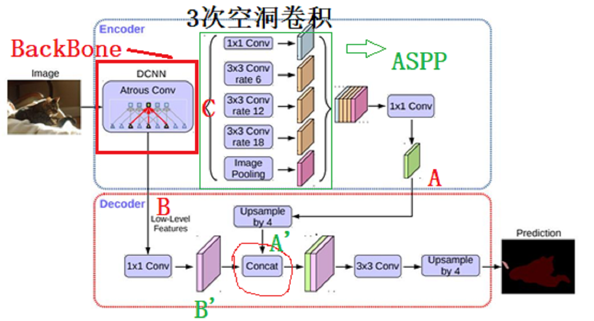
图1 网络框架图
二、BackBone
打开文件modeling.py文件,如下图:
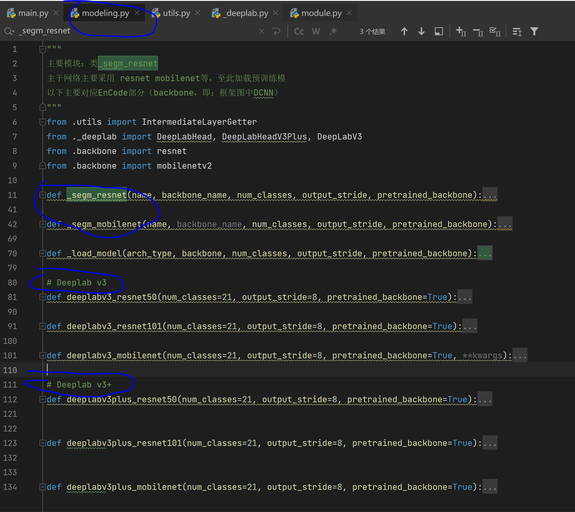
如上图,最下面6个函数表述读取6各种backbone各自的预训练模型,最上面的_segm_resnet、_segm_mobilenet表示对这6种backbone输出的多尺度特征图作处理,具体处理就是:拿出最高层、最低层特征图。在_deeplab.py文件中,我们以_segm_resnet()函数为例子,将resnet输出特征图中的其中两组重命名为: 'out'(如图1中B), 'low_level'(如图1中C),便于后续拿出。
 1 def _segm_resnet(name, backbone_name, num_classes, output_stride, pretrained_backbone):
 2
 3     if output_stride==8:
 4         replace_stride_with_dilation=[False, True, True]
 5         aspp_dilate = [12, 24, 36]  # 空洞卷积倍率
 6     else:
 7         replace_stride_with_dilation=[False, False, True]
 8         aspp_dilate = [6, 12, 18]   # 如图1,空洞卷积倍率
 9
10     backbone = resnet.__dict__[backbone_name](
11         pretrained=pretrained_backbone,
12         replace_stride_with_dilation=replace_stride_with_dilation)
13
14     inplanes = 2048
15     low_level_planes = 256
16
17     if name=='deeplabv3plus':
18         # eg:resnet输出5个尺度的特征图:layer1 layer2 layer3 layer4 layer5
19         # low_level:对应框架图中的B
20         # out:对应框架图中的C
21         return_layers = {'layer4': 'out', 'layer1': 'low_level'}
22         classifier = DeepLabHeadV3Plus(inplanes, low_level_planes, num_classes, aspp_dilate)
23     elif name=='deeplabv3':
24         return_layers = {'layer4': 'out'}
25         classifier = DeepLabHead(inplanes , num_classes, aspp_dilate)
26     # 提取网络的第几层输出结果并给一个别名
27     backbone = IntermediateLayerGetter(backbone, return_layers=return_layers)
28
29     model = DeepLabV3(backbone, classifier)
30     return model
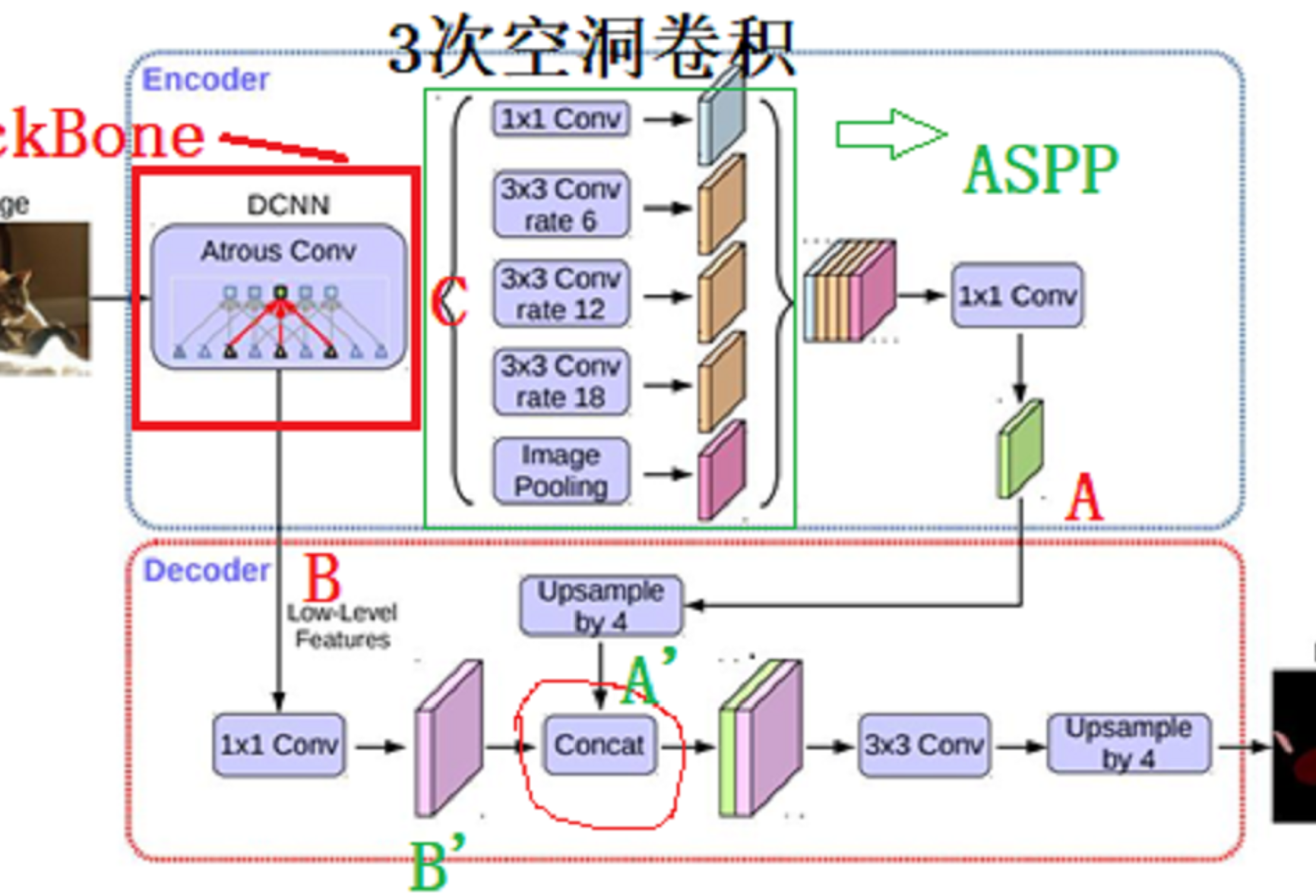
上面已经解释了如果拿到特征C、B,如下图,C由ASPP得到A,A经过4倍上采样得到A‘。B经过处理后得到B’,然后和A一起concat,然后作后面的处理。
三、Neck:ASPP
3.1 空洞卷积
越难预测的样本,往往需要更加全局的信息,空洞卷积提取大视野特征,可解决这个问题。
略
2014年 FCN
Xxxx年 DeepLabV3+(增加空洞卷积,增加感受野)
空洞卷积的优势:
- 图像分割任务中(其他场景也适用)需要较大感受野来更好完成任务
- 通过设置dilation rate参数来完成空洞卷积,并没有额外计算
- 可以按照参数扩大任意倍数的感受野,而且没有引入额外的参数
- 应用简单,就是卷积层中多设置一个参数就可以了
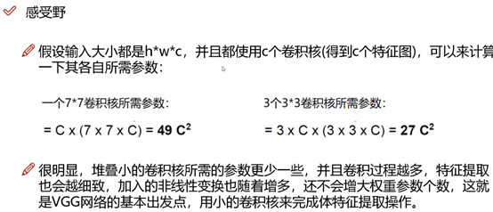
3.2 感受野
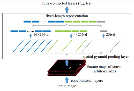
3.3 SPP(Spital pyramid pooling)
我在博客:yolov5中讲解过:https://www.cnblogs.com/winslam/p/14452136.html 但是当时理解深度不够,这里补充下:当网络中有FC层,此时输入图像分辨率必须是固定的;而当网络FC前接一个SPP层后,则输入图像分辨率将不在有任何限制。如下图,任意分辨率的图像经过卷积层后,分三条路走,分别是经过4*4、2*2、1*1的pooling,将得到16*256、4*256、1*256的特征图,然后concat一起,得到(16+4+1)*256的特征图,后续连接FC层。
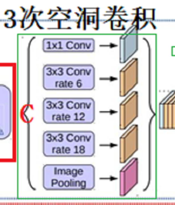
3.4 ASPP(atrous conv SPP)
ASPP差不多就是将SPP中的Pooling换成了空洞卷积,在文件_deeplab.py中,类ASPP代码如下:红色注释对应下图中ASPP的5个步骤:
 1 # 如上图:输入特征C,输出特征A
 2 class ASPP(nn.Module):
 3     def __init__(self, in_channels, atrous_rates):
 4         super(ASPP, self).__init__()
 5         out_channels = 256
 6         modules = []
 7         # 1×1 Conv
 8         modules.append(nn.Sequential(
 9             nn.Conv2d(in_channels, out_channels, 1, bias=False),
10             nn.BatchNorm2d(out_channels),
11             nn.ReLU(inplace=True)))
12
13         rate1, rate2, rate3 = tuple(atrous_rates)
14         # 3×3 Conv rate6
15         modules.append(ASPPConv(in_channels, out_channels, rate1))
16         # 3×3 Conv rate12
17         modules.append(ASPPConv(in_channels, out_channels, rate2))
18         # 3×3 Conv rate18
19         modules.append(ASPPConv(in_channels, out_channels, rate3))
20         # Image Pooling
21         modules.append(ASPPPooling(in_channels, out_channels))
22
23         self.convs = nn.ModuleList(modules)
24
25         self.project = nn.Sequential(
26             nn.Conv2d(5 * out_channels, out_channels, 1, bias=False),
27             nn.BatchNorm2d(out_channels),
28             nn.ReLU(inplace=True),
29             nn.Dropout(0.1),)
30
31     def forward(self, x):
32         res = []
33         for conv in self.convs:
34             #print(conv(x).shape)
35             res.append(conv(x))
36         res = torch.cat(res, dim=1)
37         return self.project(res)
四、Head:DeepLabHead
网络的head部分写在_deeplab.py文件中的类DeepLabHeadV3Plus,从代码看,Head部分包括如下图蓝圈部分,即:由B、C得到A‘、B’,之后concat+conv得到D,网络最后的“UpSample by 4”在文件utils.py中的类_SimpleSegmentationModel。
 1 class DeepLabHeadV3Plus(nn.Module):
 2     def __init__(self, in_channels, low_level_channels, num_classes, aspp_dilate=[12, 24, 36]):
 3         super(DeepLabHeadV3Plus, self).__init__()
 4         self.project = nn.Sequential(
 5             nn.Conv2d(low_level_channels, 48, 1, bias=False), # 实验证明48比64好
 6             nn.BatchNorm2d(48),
 7             nn.ReLU(inplace=True),
 8         )
 9
10         self.aspp = ASPP(in_channels, aspp_dilate)
11
12         self.classifier = nn.Sequential(
13             nn.Conv2d(304, 256, 3, padding=1, bias=False),
14             nn.BatchNorm2d(256),
15             nn.ReLU(inplace=True),
16             nn.Conv2d(256, num_classes, 1)
17         )
18         self._init_weight()
19
20     def forward(self, feature):
21         # feature:见modeling.py文件中第28行
22         # low_level:对应上图中的B
23         # out:对应上图中的C
24         #
25         # B -> B‘
26         low_level_feature = self.project( feature['low_level'] )#return_layers = {'layer4': 'out', 'layer1': 'low_level'}
27         #print(low_level_feature.shape)
28         # ASSP:C -> A
29         output_feature = self.aspp(feature['out'])
30         #print(output_feature.shape)
31         # (UpSample by 4):A -> A'
32         output_feature = F.interpolate(output_feature, size=low_level_feature.shape[2:], mode='bilinear', align_corners=False)
33         #print(output_feature.shape)
34         # concat(A',B') & 3*3 Conv
35         return self.classifier( torch.cat( [ low_level_feature, output_feature ], dim=1 ) )
36
37     def _init_weight(self):
38         for m in self.modules():
39             if isinstance(m, nn.Conv2d):
40                 nn.init.kaiming_normal_(m.weight)
41             elif isinstance(m, (nn.BatchNorm2d, nn.GroupNorm)):
42                 nn.init.constant_(m.weight, 1)
43                 nn.init.constant_(m.bias, 0)
五、性能评估
学习下得了
六、性能评估
由于代码使用了预训练模型,例如mobilenet resnet Xception等作为BackBone提取特征,这部分网络没有在代码中定义,代码中定义的只有ASSP和EnCoder部分,所以torch_script导出的模型之后后半部分,这个有点蛋疼,暂时就懒得折腾了。

 浙公网安备 33010602011771号