

Elasticsearch 中的 Bucket
Elasticsearch 除了在搜索方面非常之快,对数据分析也是非常重要的一面。正确理解 Bucket Aggregation 对我们使用 Kibana 非常重要。Elasticsearch 提供了非常多的 Aggregation 可以供我们使用。其中 Bucket aggregation 对于初学者来说也是比较不容易理解的一个。在今天的这篇文章中,我来重点讲述这个。
原文地址:https://blog.csdn.net/UbuntuTouch/article/details/103679273
透彻理解 Elasticsearch 中的 Bucket Aggregation
简单地说:一个桶代表一个具有共同标准的文档集合。存储桶(bucket)是聚合的关键要素。比如,我们想分析每个月的 log 流量: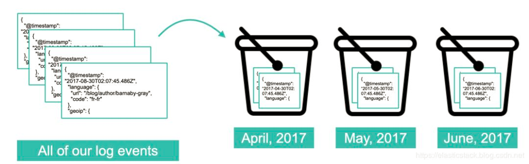
存储桶聚合(bucket Aggregation)不像指标聚合(Metric Aggregation)那样计算字段的指标,而是创建文档存储桶。每个存储桶都与一个标准(取决于聚合类型)相关联,该标准确定当前上下文中的文档是否“落入”其中。换句话说,存储桶有效地定义了文档集。除了存储桶本身之外,存储桶聚合还计算并返回落入每个存储桶的文档数量。
与指标聚合相反,存储桶聚合可以保存子聚合。这些子聚合将针对其“父”存储桶聚合创建的存储桶进行聚合。
有不同的存储桶聚合器,每个聚合器都有不同的“存储桶”策略。一些定义单个存储桶,一些定义固定数量的多个存储桶,另一些定义在聚合过程中动态创建存储桶。
尽管存储桶聚合不计算指标,但它们可以包含可以为存储桶聚合生成的每个存储桶计算指标的指标子聚合。这使存储桶聚合对于粒度表示和分析 Elasticsearch 索引非常有用。在本文中,我们将重点介绍直方图(histogram),范围(range),过滤器(filter)和术语(terms)等存储桶聚合。让我们开始吧!
什么是桶?
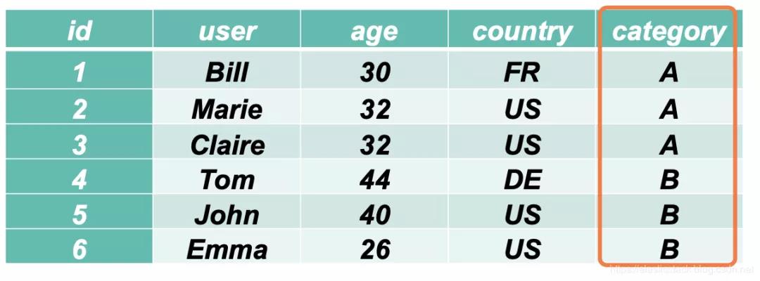
首先为了说明问题的方便,我们来展示一个简单的 SpreadSheet 表格:
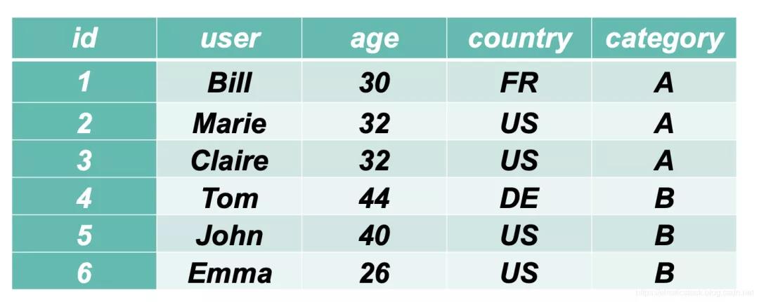
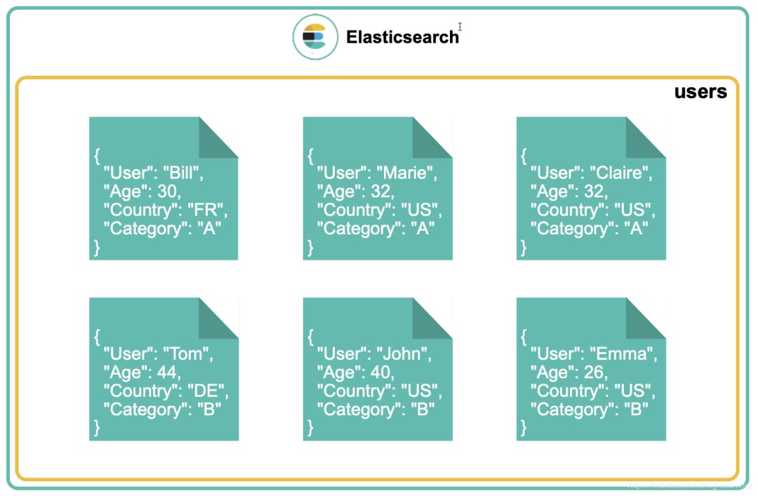
在上面的表格中,我们可以看到一个很规整的关于用户的名单。每天用户具有 id,user,age,country 及 category。当这些数据被存于到 Elasticsearch 中后,会变成一个一个的文档:
假如我们想得到这些个用户的平均年龄,我们很容易通过 Elasticsearch 的 Avg Aggregation 来得到。
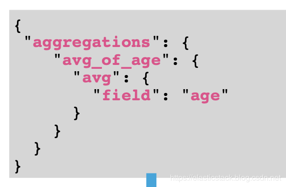

那么他们的平均年龄是34岁。
接下来我们开始谈我们的重点了:Bucket Aggregation。
简单地说:Bucket Aggregation 是一种把具有相同标准的数据分组数据的方法。创建存储桶:
收集具有共同标准的文件
‒可以具有一个或多个与其关联的指标
bucket 每个存储桶的文档数(文档数)是默认指标
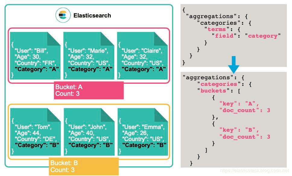
首先,我们可以按照 cetegory 进行分类:
我们从上面的表格可以看出来 category A 有 3 个文档,而 category B 有 3 个文档。
上面我们得到了每个 category 的数量是我们想要的,但是在很多的情况下,我们更想得到在这每天 category 下的一些指标,比如每个 category 的平均年龄是多少?这样我实际上是在以 category 为 key 的存储桶里来求平均值。
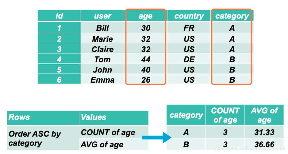
我们可以通过如下的方法来得到这个:

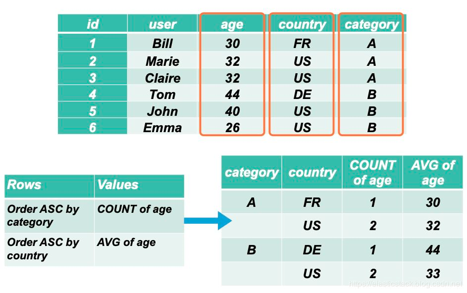
这样,我们就得到了在每个 category 下的平均年龄。我们可以再进一步想得到在每个 category 下的每个国家的平均年龄。显然这个时候,我们需要使用到 country这个桶,这桶是在 category 桶下面的另外一个桶。
如果大家对上面的实验有兴趣,可以把如下的数据导入到 Elasticsearch 中:
1 2 3 4 5 6 7 8 9 10 11 12 13 14 15 16 17 18 19 | PUT users{ "mappings": { "properties": { "age": { "type": "long" }, "category": { "type": "keyword" }, "country": { "type": "keyword" }, "user": { "type": "keyword" } } }} |
我们使用 Bulk API 来导入数据:
1 2 3 4 5 6 7 8 9 10 11 12 13 | POST _bulk{ "index" : { "_index" : "users", "_id": 1} }{"user":"bill", "age": 30, "country": "FR", "category": "A"}{ "index" : { "_index" : "users", "_id": 2} }{"user":"Marie", "age": 32, "country": "US", "category": "A"}{ "index" : { "_index" : "users", "_id": 3} }{"user":"Clarie", "age": 32, "country": "US", "category": "A"}{ "index" : { "_index" : "users", "_id": 4} }{"user":"Tom", "age": 44, "country": "DE", "category": "B"}{ "index" : { "_index" : "users", "_id": 5} }{"user":"John", "age": 40, "country": "US", "category": "B"}{ "index" : { "_index" : "users", "_id": 6} }{"user":"Emma", "age": 26, "country": "US", "category": "B"} |
最后一步的查询:
1 2 3 4 5 6 7 8 9 10 11 12 13 14 15 16 17 18 19 20 21 22 23 24 25 | GET users/_search{ "size": 0, "aggs": { "categories": { "terms": { "field": "category" }, "aggs": { "countries": { "terms": { "field": "country" }, "aggs": { "average_age": { "avg": { "field": "age" } } } } } } }} |
显示结果:


 1 {
 2   "took" : 2,
 3   "timed_out" : false,
 4   "_shards" : {
 5     "total" : 1,
 6     "successful" : 1,
 7     "skipped" : 0,
 8     "failed" : 0
 9   },
10   "hits" : {
11     "total" : {
12       "value" : 6,
13       "relation" : "eq"
14     },
15     "max_score" : null,
16     "hits" : [ ]
17   },
18   "aggregations" : {
19     "categories" : {
20       "doc_count_error_upper_bound" : 0,
21       "sum_other_doc_count" : 0,
22       "buckets" : [
23         {
24           "key" : "A",
25           "doc_count" : 3,
26           "countries" : {
27             "doc_count_error_upper_bound" : 0,
28             "sum_other_doc_count" : 0,
29             "buckets" : [
30               {
31                 "key" : "US",
32                 "doc_count" : 2,
33                 "average_age" : {
34                   "value" : 32.0
35                 }
36               },
37               {
38                 "key" : "FR",
39                 "doc_count" : 1,
40                 "average_age" : {
41                   "value" : 30.0
42                 }
43               }
44             ]
45           }
46         },
47         {
48           "key" : "B",
49           "doc_count" : 3,
50           "countries" : {
51             "doc_count_error_upper_bound" : 0,
52             "sum_other_doc_count" : 0,
53             "buckets" : [
54               {
55                 "key" : "US",
56                 "doc_count" : 2,
57                 "average_age" : {
58                   "value" : 33.0
59                 }
60               },
61               {
62                 "key" : "DE",
63                 "doc_count" : 1,
64                 "average_age" : {
65                   "value" : 44.0
66                 }
67               }
68             ]
69           }
70         }
71       ]
72     }
73   }
74 }
在这一节里,我们主要通过 terms Aggregation 来展示存储桶的概念。我在下面用一个具体的例子来详细描述更多桶的操作。
准备数据
为了说明介绍中提到的各种存储桶聚合,我们首先创建一个新的 “sports” 索引,该索引存储 “althlete” 文档的集合。索引映射将包含诸如运动员的位置,姓名,等级,运动,年龄,进球数和场位置(例如防守者)之类的字段。让我们创建映射:
1 2 3 4 5 6 7 8 9 10 11 12 13 14 15 16 17 18 19 20 21 22 23 24 25 26 27 28 29 30 31 32 33 34 35 | PUT sports{ "mappings": { "properties": { "birthdate": { "type": "date", "format": "dateOptionalTime" }, "location": { "type": "geo_point" }, "name": { "type": "keyword" }, "rating": { "type": "integer" }, "sport": { "type": "keyword" }, "age": { "type": "integer" }, "goals": { "type": "integer" }, "role": { "type": "keyword" }, "score_weight": { "type": "float" } } }} |
一旦 mapping 创建成功,我们就可以使用 Elasticsearch 所提供的 Bulk API 来把我们数据导入到我们的索引中。我们可以通过一个 REST 调用就把所有的数据导入到 Elasticsearch 中。
1 2 3 4 5 6 7 8 9 10 11 12 13 14 15 16 17 18 19 20 21 22 23 24 25 26 27 28 29 30 31 32 33 34 35 36 37 38 39 40 41 42 43 44 45 | POST sports/_bulk{"index":{"_index":"sports"}}{"name":"Michael","birthdate":"1989-10-1","sport":"Football","rating":["5","4"],"location":"46.22,-68.45","age":"23","goals":"43","score_weight":"3","role":"midfielder"}{"index":{"_index":"sports"}}{"name":"Bob","birthdate":"1989-11-2","sport":"Football","rating":["3","4"],"location":"45.21,-68.35","age":"33","goals":"54","score_weight":"2","role":"forward"}{"index":{"_index":"sports"}}{"name":"Jim","birthdate":"1988-10-3","sport":"Football","rating":["3","2"],"location":"45.16,-63.58","age":"28","goals":"73","score_weight":"2","role":"forward"}{"index":{"_index":"sports"}}{"name":"Joe","birthdate":"1992-5-20","sport":"Basketball","rating":["4","3"],"location":"45.22,-68.53","age":"18","goals":"848","score_weight":"3","role":"midfielder"}{"index":{"_index":"sports"}}{"name":"Tim","birthdate":"1992-2-28","sport":"Basketball","rating":["3","3"],"location":"46.22,-68.85","age":"28","goals":"942","score_weight":"2","role":"forward"}{"index":{"_index":"sports"}}{"name":"Alfred","birthdate":"1990-9-9","sport":"Football","rating":["2","2"],"location":"45.12,-68.35","age":"25","goals":"53","score_weight":"4","role":"defender"}{"index":{"_index":"sports"}}{"name":"Jeff","birthdate":"1990-4-1","sport":"Hockey","rating":["2","3"],"location":"46.12,-68.55","age":"26","goals":"93","score_weight":"3","role":"midfielder"}{"index":{"_index":"sports"}}{"name":"Will","birthdate":"1988-3-1","sport":"Hockey","rating":["4","4"],"location":"46.25,-84.25","age":"27","goals":"124","score_weight":"2","role":"forward"}{"index":{"_index":"sports"}}{"name":"Mick","birthdate":"1989-10-1","sport":"Football","rating":["3","4"],"location":"46.22,-68.45","age":"35","goals":"56","score_weight":"3","role":"midfielder"}{"index":{"_index":"sports"}}{"name":"Pong","birthdate":"1989-11-2","sport":"Basketball","rating":["1","3"],"location":"45.21,-68.35","age":"34","goals":"1483","score_weight":"2","role":"forward"}{"index":{"_index":"sports"}}{"name":"Ray","birthdate":"1988-10-3","sport":"Football","rating":["2","2"],"location":"45.16,-63.58","age":"31","goals":"84","score_weight":"3","role":"midfielder"}{"index":{"_index":"sports"}}{"name":"Ping","birthdate":"1992-5-20","sport":"Basketball","rating":["4","3"],"location":"45.22,-68.53","age":"27","goals":"1328","score_weight":"2","role":"forward"}{"index":{"_index":"sports"}}{"name":"Duke","birthdate":"1992-2-28","sport":"Hockey","rating":["5","2"],"location":"46.22,-68.85","age":"41","goals":"218","score_weight":"2","role":"forward"}{"index":{"_index":"sports"}}{"name":"Hal","birthdate":"1990-9-9","sport":"Hockey","rating":["4","2"],"location":"45.12,-68.35","age":"18","goals":"148","score_weight":"3","role":"midfielder"}{"index":{"_index":"sports"}}{"name":"Charge","birthdate":"1990-4-1","sport":"Football","rating":["3","2"],"location":"44.19,-82.55","age":"19","goals":"34","score_weight":"4","role":"defender"}{"index":{"_index":"sports"}}{"name":"Barry","birthdate":"1988-3-1","sport":"Football","rating":["5","2"],"location":"36.45,-79.15","age":"20","goals":"48","score_weight":"4","role":"defender"}{"index":{"_index":"sports"}}{"name":"Bank","birthdate":"1988-3-1","sport":"Handball","rating":["6","4"],"location":"46.25,-54.53","age":"25","goals":"150","score_weight":"4","role":"defender"}{"index":{"_index":"sports"}}{"name":"Bingo","birthdate":"1988-3-1","sport":"Handball","rating":["10","7"],"location":"46.25,-68.55","age":"29","goals":"143","score_weight":"3","role":"midfielder"}{"index":{"_index":"sports"}}{"name":"James","birthdate":"1988-3-1","sport":"Basketball","rating":["10","8"],"location":"41.25,-69.55","age":"36","goals":"1284","score_weight":"2","role":"forward"}{"index":{"_index":"sports"}}{"name":"Wayne","birthdate":"1988-3-1","sport":"Hockey","rating":["10","10"],"location":"46.21,-68.55","age":"25","goals":"113","score_weight":"3","role":"midfielder"}{"index":{"_index":"sports"}}{"name":"Brady","birthdate":"1988-3-1","sport":"Handball","rating":["10","10"],"location":"63.24,-84.55","age":"29","goals":"443","score_weight":"2","role":"forward"}{"index":{"_index":"sports"}}{"name":"Lewis","birthdate":"1988-3-1","sport":"Football","rating":["10","10"],"location":"56.25,-74.55","age":"24","goals":"49","score_weight":"3","role":"midfielder"} |
这样我们的数据就录入到 Elasticsearch 中了。在下面,我们就用不同的存储桶来对我们的数据进行统计。
Filter(s) Aggregation
桶聚合支持单过滤器聚合和多过滤器聚合。
单个过滤器聚合根据与过滤器定义中指定的查询或字段值匹配的所有文档构造单个存储桶。当您要标识一组符合特定条件的文档时,单过滤器聚合很有用。
例如,我们可以使用单过滤器聚合来查找所有具有 “defender” 角色的运动员,并计算每个过滤桶的平均目标。过滤器配置如下所示:
1 2 3 4 5 6 7 8 9 10 11 12 13 14 15 16 17 18 19 20 | POST sports/_search{ "size": 0, "aggs": { "defender_filter": { "filter": { "term": { "role": "defender" } }, "aggs": { "avg_goals": { "avg": { "field": "goals" } } } } }} |
我们看到的结果是:
1 2 3 4 5 6 7 8 | "aggregations" : { "defender_filter" : { "doc_count" : 4, "avg_goals" : { "value" : 71.25 } } } |
如您所见,filter 聚合包含一个 “term” 字段,该字段指定文档中的字段以搜索特定值(在本例中为 “defender”)。Elasticsearch 将遍历所有文档,并检查 “role” 字段中是否包含 “defender”。然后将与该值匹配的文档添加到聚合生成的单个存储桶中。此输出表明我们集合中所有后卫的平均进球数为 71.25。
这是单过滤器聚合的示例。但是,在 Elasticsearch 中,您可以选择使用 filter 聚合指定多个过滤器。这是一个多值聚合,其中每个存储桶都对应一个特定的过滤器。我们可以修改上面的示例以过滤 defender 和 foward:
1 2 3 4 5 6 7 8 9 10 11 12 13 14 15 16 17 18 19 20 21 22 23 24 25 26 27 28 29 | GET sports/_search{ "size": 0, "aggs": { "athletes": { "filters": { "filters": { "defenders": { "term": { "role": "defender" } }, "forwards": { "term": { "role": "forward" } } } }, "aggs": { "avg_goals": { "avg": { "field": "goals" } } } } }} |
显示结果为:
1 2 3 4 5 6 7 8 9 10 11 12 13 14 15 16 17 18 | "aggregations" : { "athletes" : { "buckets" : { "defenders" : { "doc_count" : 4, "avg_goals" : { "value" : 71.25 } }, "forwards" : { "doc_count" : 9, "avg_goals" : { "value" : 661.0 } } } }} |
我们可以看出来我们同时有两个桶,分别对应我们的两个 filter。每一个 filter 都检查 role 的值为 defender 或者 forward。
Terms Aggregation
也许我们对 Terms Aggregation 并不陌生。我们刚才在一开始已经使用了 Terms Aggregation。
术语聚合会在文档的指定字段中搜索唯一值,并为找到的每个唯一值构建存储桶。与过滤器聚合不同,术语聚合的任务不是将结果限制为特定值,而是查找文档中给定字段的所有唯一值。
看一下下面的示例,我们试图为 “sport” 字段中找到的每个唯一值创建一个存储桶。这项操作的结果是,我们将为索引中的每种运动提供四个独特的存储桶:Football,Handball,Hockey 和 Basketbalk。然后,我们将使用平均子聚合计算每种运动的平均目标:
1 2 3 4 5 6 7 8 9 10 11 12 13 14 15 16 17 18 | GET sports/_search{ "size": 0, "aggs": { "sports": { "terms": { "field": "sport" }, "aggs": { "avg_scoring": { "avg": { "field": "goals" } } } } }} |
返回数据为:
1 2 3 4 5 6 7 8 9 10 11 12 13 14 15 16 17 18 19 20 21 22 23 24 25 26 27 28 29 30 31 32 33 34 35 36 | "aggregations" : { "sports" : { "doc_count_error_upper_bound" : 0, "sum_other_doc_count" : 0, "buckets" : [ { "key" : "Football", "doc_count" : 9, "avg_scoring" : { "value" : 54.888888888888886 } }, { "key" : "Basketball", "doc_count" : 5, "avg_scoring" : { "value" : 1177.0 } }, { "key" : "Hockey", "doc_count" : 5, "avg_scoring" : { "value" : 139.2 } }, { "key" : "Handball", "doc_count" : 3, "avg_scoring" : { "value" : 245.33333333333334 } } ] } } |
如您所见,术语聚合为索引中的每种运动类型构造了四个存储桶。每个存储桶包含doc_count(属于存储桶的文档数)和每个运动的平均子聚合。
Histogram Aggregation
直方图聚合使我们可以根据指定的时间间隔构造存储桶。属于每个间隔的值将形成一个间隔存储桶。例如,假设我们要使用5年间隔将直方图聚合应用于 “age” 字段。在这种情况下,直方图聚合将在我们的文档集中找到最小和最大年龄,并将每个文档与指定的时间间隔相关联。每个文档的 “age” 字段将向下舍入到最接近的时间间隔存储桶。例如,假设我们的时间间隔值为 5,存储分区大小为 6,则年龄 32会四舍五入为 30。
直方图聚合的公式如下所示:
bucket_key = Math.floor((value - offset) / interval) * interval + offset
请注意,时间间隔必须为正十进制数,而偏移量必须为 [0,offset] 范围内的十进制。
让我们使用直方图聚合来生成篮球中目标间隔为 200 的存储桶。
1 2 3 4 5 6 7 8 9 10 11 12 13 14 15 16 17 18 19 20 21 | POST sports/_search{ "size": 0, "aggs": { "baskketball_filter": { "filter": { "term": { "sport": "Basketball" } }, "aggs": { "goals_histogram": { "histogram": { "field": "goals", "interval": 200 } } } } }} |
返回结果:
1 2 3 4 5 6 7 8 9 10 11 12 13 14 15 16 17 18 19 20 21 22 23 24 25 | "aggregations" : { "baskketball_filter" : { "doc_count" : 5, "goals_histogram" : { "buckets" : [ { "key" : 800.0, "doc_count" : 2 }, { "key" : 1000.0, "doc_count" : 0 }, { "key" : 1200.0, "doc_count" : 2 }, { "key" : 1400.0, "doc_count" : 1 } ] } } } |
上面的回答表明,没有目标落在 0-200、200-400、400-600 和 600-800 区间内。因此,第一个存储区从 800-1000 间隔开始。因此,值最小的文档将确定最小存储桶(最小 key 的存储桶)。相应地,具有最高值的文档将确定最大存储桶(具有最高 key 的存储桶)。
此外,该响应还显示有零个文档落在 [1000,1200)范围内。这意味着没有运动员得分在 1000 到 1200 个目标之间。默认情况下,Elasticsearch 用空存储桶填充此类空白。您可以使用min_doc_count 设置通过请求最小计数不为零的存储桶来更改此行为。例如,如果我们将min_doc_count 的值设置为 1,则直方图将仅针对其中包含不少于 1 个文档的间隔构造存储桶。让我们修改查询,将 min_doc_count 设置为1。
1 2 3 4 5 6 7 8 9 10 11 12 13 14 15 16 17 18 19 20 21 22 | POST sports/_search{ "size": 0, "aggs": { "baskketball_filter": { "filter": { "term": { "sport": "Basketball" } }, "aggs": { "goals_histogram": { "histogram": { "field": "goals", "interval": 200, "min_doc_count": 1 } } } } }} |
那么经过这样修改后的返回结果是:
1 2 3 4 5 6 7 8 9 10 11 12 13 14 15 16 17 18 19 20 21 | "aggregations" : { "baskketball_filter" : { "doc_count" : 5, "goals_histogram" : { "buckets" : [ { "key" : 800.0, "doc_count" : 2 }, { "key" : 1200.0, "doc_count" : 2 }, { "key" : 1400.0, "doc_count" : 1 } ] } } } |
我们还可以使用 extended_bounds 设置来强制直方图聚合,以根据特定的最小值开始构建其存储桶,并继续构建存储桶直至达到最大值(即使不再有文档)。仅当将 min_doc_count 设置为0时,才使用 extended_bounds。(如果min_doc_count 大于0,则不会返回空存储桶)。看一下这个查询:
1 2 3 4 5 6 7 8 9 10 11 12 13 14 15 16 17 18 19 20 21 22 23 24 25 26 | POST sports/_search{ "size": 0, "aggs": { "baskketball_filter": { "filter": { "term": { "sport": "Basketball" } }, "aggs": { "goals_histogram": { "histogram": { "field": "goals", "interval": 200, "min_doc_count": 0, "extended_bounds": { "min": 0, "max": 1600 } } } } } }} |
在这里,我们为存储桶指定了 0(最小值)和 1600(最大值)。因此,响应应如下所示:
1 2 3 4 5 6 7 8 9 10 11 12 13 14 15 16 17 18 19 20 21 22 23 24 25 26 27 28 29 30 31 32 33 34 35 36 37 38 39 40 41 42 43 44 45 | "aggregations" : { "baskketball_filter" : { "doc_count" : 5, "goals_histogram" : { "buckets" : [ { "key" : 0.0, "doc_count" : 0 }, { "key" : 200.0, "doc_count" : 0 }, { "key" : 400.0, "doc_count" : 0 }, { "key" : 600.0, "doc_count" : 0 }, { "key" : 800.0, "doc_count" : 2 }, { "key" : 1000.0, "doc_count" : 0 }, { "key" : 1200.0, "doc_count" : 2 }, { "key" : 1400.0, "doc_count" : 1 }, { "key" : 1600.0, "doc_count" : 0 } ] } } } |
如您所见,即使第一个存储桶和最后一个存储桶根本没有任何值,也会生成从 0 到结束 1600 的所有存储桶。
Date Histogram Aggregation
我们可以使用 date histogram aggregation 来统计我们的运动员出生年月分别情况:
1 2 3 4 5 6 7 8 9 10 11 12 | GET sports/_search{ "size": 0, "aggs": { "birthdays": { "date_histogram": { "field": "birthdate", "interval": "year" } } }} |
返回的结果是:
1 2 3 4 5 6 7 8 9 10 11 12 13 14 15 16 17 18 19 20 21 22 23 24 25 26 27 28 29 30 31 | "aggregations" : { "birthdays" : { "buckets" : [ { "key_as_string" : "1988-01-01T00:00:00.000Z", "key" : 567993600000, "doc_count" : 10 }, { "key_as_string" : "1989-01-01T00:00:00.000Z", "key" : 599616000000, "doc_count" : 4 }, { "key_as_string" : "1990-01-01T00:00:00.000Z", "key" : 631152000000, "doc_count" : 4 }, { "key_as_string" : "1991-01-01T00:00:00.000Z", "key" : 662688000000, "doc_count" : 0 }, { "key_as_string" : "1992-01-01T00:00:00.000Z", "key" : 694224000000, "doc_count" : 4 } ] } } |
上面的结果显示在 1988 年到 1998 年之间的运动员有 10 个,在 1989 和 1990 年之间的有 4 位。
当然我们也可以针对每个年龄段的 goals 的平均值:
1 2 3 4 5 6 7 8 9 10 11 12 13 14 15 16 17 18 19 | GET sports/_search{ "size": 0, "aggs": { "birthdays": { "date_histogram": { "field": "birthdate", "interval": "year" }, "aggs": { "average_goals": { "avg": { "field": "goals" } } } } }} |
返回的结果是:
1 2 3 4 5 6 7 8 9 10 11 12 13 14 15 16 17 18 19 20 21 22 23 24 25 26 27 28 29 30 31 32 33 34 35 36 37 38 39 40 41 42 43 44 45 46 | "aggregations" : { "birthdays" : { "buckets" : [ { "key_as_string" : "1988-01-01T00:00:00.000Z", "key" : 567993600000, "doc_count" : 10, "average_goals" : { "value" : 251.1 } }, { "key_as_string" : "1989-01-01T00:00:00.000Z", "key" : 599616000000, "doc_count" : 4, "average_goals" : { "value" : 409.0 } }, { "key_as_string" : "1990-01-01T00:00:00.000Z", "key" : 631152000000, "doc_count" : 4, "average_goals" : { "value" : 82.0 } }, { "key_as_string" : "1991-01-01T00:00:00.000Z", "key" : 662688000000, "doc_count" : 0, "average_goals" : { "value" : null } }, { "key_as_string" : "1992-01-01T00:00:00.000Z", "key" : 694224000000, "doc_count" : 4, "average_goals" : { "value" : 834.0 } } ] } } |
我们可以看到在 1992 年的这个年龄段的 average_goals 是最高的,达到 834。也许是后生可畏啊!
Range Aggregation
通过此存储桶聚合,可以轻松根据用户定义的范围构建存储桶。Elasticsearch 将检查从您指定的数字字段中提取的每个值,并将其与范围进行比较,然后将该值放入相应的范围。请注意,此聚合包括起始值,但不包括每个范围的起始值。
让我们为运动索引中的 “age” 字段创建一个范围汇总:
1 2 3 4 5 6 7 8 9 10 11 12 13 14 15 16 17 18 19 20 21 22 23 | GET sports/_search{ "size": 0, "aggs": { "goal_ranges": { "range": { "field": "age", "ranges": [ { "to": 20 }, { "from": 20, "to": 30 }, { "from": 30 } ] } } }} |
如您所见,我们为查询指定了三个范围。这意味着 Elasticsearch 将创建与每个范围相对应的三个存储桶。上面的查询应产生以下输出:
1 2 3 4 5 6 7 8 9 10 11 12 13 14 15 16 17 18 19 20 21 22 | "aggregations" : { "goal_ranges" : { "buckets" : [ { "key" : "*-20.0", "to" : 20.0, "doc_count" : 3 }, { "key" : "20.0-30.0", "from" : 20.0, "to" : 30.0, "doc_count" : 13 }, { "key" : "30.0-*", "from" : 30.0, "doc_count" : 6 } ] } } |
如输出所示,我们指数中最多的运动员年龄在20至30岁之间。
为了使范围更易理解,我们可以为每个范围自定义键名,如下所示:
1 2 3 4 5 6 7 8 9 10 11 12 13 14 15 16 17 18 19 20 21 22 23 24 25 26 | GET sports/_search{ "size": 0, "aggs": { "goal_ranges": { "range": { "field": "age", "ranges": [ { "key": "start-of-career", "to": 20 }, { "key": "mid-of-career", "from": 20, "to": 30 }, { "key": "end-of-cereer", "from": 30 } ] } } }} |
这样产生的结果是:
1 2 3 4 5 6 7 8 9 10 11 12 13 14 15 16 17 18 19 20 21 22 | "aggregations" : { "goal_ranges" : { "buckets" : [ { "key" : "start-of-career", "to" : 20.0, "doc_count" : 3 }, { "key" : "mid-of-career", "from" : 20.0, "to" : 30.0, "doc_count" : 13 }, { "key" : "end-of-cereer", "from" : 30.0, "doc_count" : 6 } ] } } |
我们可以使用统计子聚合将更多信息添加到范围。此汇总将为每个范围提供最小值,最大值,平均值和总和。让我们来看看:
1 2 3 4 5 6 7 8 9 10 11 12 13 14 15 16 17 18 19 20 21 22 23 24 25 26 27 28 29 30 31 32 33 | GET sports/_search{ "size": 0, "aggs": { "goal_ranges": { "range": { "field": "age", "ranges": [ { "key": "start-of-career", "to": 20 }, { "key": "mid-of-career", "from": 20, "to": 30 }, { "key": "end-of-cereer", "from": 30 } ] }, "aggs": { "age_stats": { "stats": { "field": "age" } } } } }} |
查询结果是:
1 2 3 4 5 6 7 8 9 10 11 12 13 14 15 16 17 18 19 20 21 22 23 24 25 26 27 28 29 30 31 32 33 34 35 36 37 38 39 40 41 42 43 | "aggregations" : { "goal_ranges" : { "buckets" : [ { "key" : "start-of-career", "to" : 20.0, "doc_count" : 3, "age_stats" : { "count" : 3, "min" : 18.0, "max" : 19.0, "avg" : 18.333333333333332, "sum" : 55.0 } }, { "key" : "mid-of-career", "from" : 20.0, "to" : 30.0, "doc_count" : 13, "age_stats" : { "count" : 13, "min" : 20.0, "max" : 29.0, "avg" : 25.846153846153847, "sum" : 336.0 } }, { "key" : "end-of-cereer", "from" : 30.0, "doc_count" : 6, "age_stats" : { "count" : 6, "min" : 31.0, "max" : 41.0, "avg" : 35.0, "sum" : 210.0 } } ] } } |
Geo Distance Aggregation
使用地理距离聚合,您可以定义一个原点和到该点的一组距离范围。然后,聚合将评估每个geo_point 值到原点的距离,并确定文档属于哪个范围。如果文档的geo_point 值与原点之间的距离落入该存储桶的距离范围内,则该文档被视为属于该存储桶。
在下面的示例中,我们的原点的纬度值为 46.22,经度值为 -68.85。我们使用原点46.22,-68.85 的字符串格式,其中第一个值定义纬度,第二个值定义经度。或者,您可以使用对象格式 -{“ lat”:46.22,“ lon”:-68.85} 或数组格式:[-68.85,46.22] 基于 GeoJson 标准,其中第一个数字是 lon 和第二个是拉特
另外,我们以 km 值创建三个范围。默认距离单位是 m(米),因此我们需要在“ unit”(单位)字段中明确设置 km。其他受支持的距离单位是 mi(英里),in(英寸),yd(码),cm(厘米)和mm(毫米)。
1 2 3 4 5 6 7 8 9 10 11 12 13 14 15 16 17 18 19 20 21 22 23 24 25 26 | POST sports/_search{ "size": 0, "aggs": { "althlete_location": { "geo_distance": { "field": "location", "origin": { "lat": 46.22, "lon": -68.85 }, "ranges": [ { "to": 200 }, { "from": 200, "to": 400 }, { "from": 400 } ] } } }} |
查询结果:
1 2 3 4 5 6 7 8 9 10 11 12 13 14 15 16 17 18 19 20 21 22 23 | "aggregations" : { "althlete_location" : { "buckets" : [ { "key" : "*-200.0", "from" : 0.0, "to" : 200.0, "doc_count" : 2 }, { "key" : "200.0-400.0", "from" : 200.0, "to" : 400.0, "doc_count" : 0 }, { "key" : "400.0-*", "from" : 400.0, "doc_count" : 20 } ] } } |
结果表明,居住在距起点不超过 200 km 的运动员有 2 名,居住在距起点超过 400 km 的运动员有 20 名。
IP Range Aggregation
Elasticsearch 还具有对 IP 范围的内置支持。IP 聚合的工作方式与其他范围聚合类似。让我们为 IP 地址创建索引映射,以说明此聚合的工作方式:
1 2 3 4 5 6 7 8 9 10 | PUT ips{ "mappings": { "properties": { "ip_addr": { "type": "ip" } } }} |
让我们将一些专用网络 IP 放入索引中。
1 2 3 4 5 6 7 8 9 10 11 12 13 14 15 16 17 18 19 20 21 | POST ips/_bulk{"index":{"_index":"ips"}}{ "ip_addr": "172.16.0.0" }{"index":{"_index":"ips"}}{ "ip_addr": "172.16.0.1" }{"index":{"_index":"ips"}}{ "ip_addr": "172.16.0.2" }{"index":{"_index":"ips"}}{ "ip_addr": "172.16.0.3" }{"index":{"_index":"ips"}}{ "ip_addr": "172.16.0.4" }{"index":{"_index":"ips"}}{ "ip_addr": "172.16.0.5" }{"index":{"_index":"ips"}}{ "ip_addr": "172.16.0.6" }{"index":{"_index":"ips"}}{ "ip_addr": "172.16.0.7" }{"index":{"_index":"ips"}}{ "ip_addr": "172.16.0.8" }{"index":{"_index":"ips"}}{ "ip_addr": "172.16.0.9" } |
现在,当索引中包含一些数据时,让我们创建一个IP范围聚合:
1 2 3 4 5 6 7 8 9 10 11 12 13 14 15 16 17 18 19 | GET ips/_search{ "size": 0, "aggs": { "ip_ranges": { "ip_range": { "field": "ip_addr", "ranges": [ { "to": "172.16.0.4" }, { "from": "172.16.0.4" } ] } } }} |
参考:https://www.elastic.co/guide/en/elasticsearch/reference/current/search-aggregations-bucket.html


【推荐】国内首个AI IDE,深度理解中文开发场景,立即下载体验Trae
【推荐】编程新体验,更懂你的AI,立即体验豆包MarsCode编程助手
【推荐】抖音旗下AI助手豆包,你的智能百科全书,全免费不限次数
【推荐】轻量又高性能的 SSH 工具 IShell:AI 加持,快人一步
· Linux系列:如何用heaptrack跟踪.NET程序的非托管内存泄露
· 开发者必知的日志记录最佳实践
· SQL Server 2025 AI相关能力初探
· Linux系列:如何用 C#调用 C方法造成内存泄露
· AI与.NET技术实操系列(二):开始使用ML.NET
· 被坑几百块钱后,我竟然真的恢复了删除的微信聊天记录!
· 没有Manus邀请码?试试免邀请码的MGX或者开源的OpenManus吧
· 【自荐】一款简洁、开源的在线白板工具 Drawnix
· 园子的第一款AI主题卫衣上架——"HELLO! HOW CAN I ASSIST YOU TODAY
· Docker 太简单,K8s 太复杂?w7panel 让容器管理更轻松!