

第四章:目标检测YoloV3(上)
目录
对计算机而言,能够“看到”的是图像被编码之后的数字,但它很难解高层语义概念,比如图像或者视频帧中出现目标的是人还是物体,更无法定位目标出现在图像中哪个区域。目标检测的主要目的是让计算机可以自动识别图片或者视频帧中所有目标的类别,并在该目标周围绘制边界框,标示出每个目标的位置,如 图1 所示。
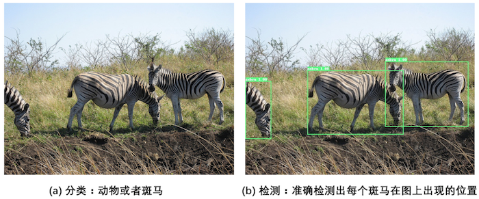
图1:图像分类和目标检测示意图
- 图1(a)是图像分类任务,只需 识别 出这是一张斑马的图片。
- 图1(b)是目标检测任务,不仅要 识别 出这是一张斑马的图片,还要 标出 图中斑马的 位置 。
目标检测发展历程
图像分类处理基本流程:
- 先使用卷积神经网络提取图像特征
- 然后再用这些特征预测分类概率
- 根据训练样本标签建立起分类损失函数
- 开启端到端的训练
如 图2 所示。
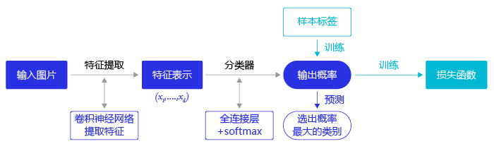
图2:图像分类流程示意图
但对于目标检测问题,按照 图2 的流程则行不通。因为在图像分类任务中,对整张图提取特征的过程中 没能体现出不同目标之间的区别 ,最终也就 没法分别标示出每个物体所在的位置 。
为了解决这个问题,结合图片分类任务取得的成功经验,我们可以将目标检测任务进行拆分。假设我们现在有某种方式可以在输入图片上生成一系列可能包含物体的区域,这些区域称为 候选区域 ,在一张图上可以生成很多个候选区域。然后对每个候选区域,可以把它单独当成一幅图像来看待,使用图像分类模型对它进行分类,看它属于哪个类别或者背景(即不包含任何物体的类别)。
上一节我们学过如何解决图像分类任务,使用卷积神经网络对一幅图像进行分类不再是一件困难的事情。那么,现在问题的关键就是如何产生候选区域?比如我们可以使用穷举法来产生候选区域,如图3所示。
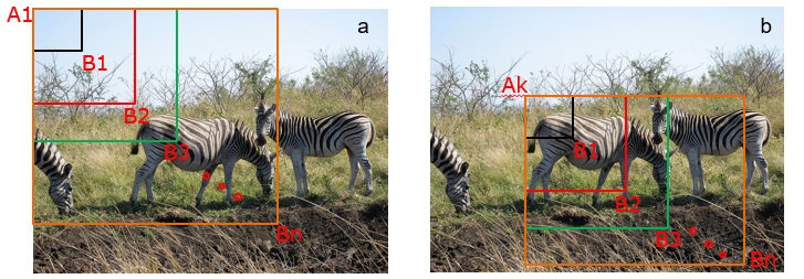
图3:候选区域
A为图像上的某个像素点,B为A右下方另外一个像素点,A、B两点可以确定一个矩形框,记作AB。
- 如图3(a)所示:A在图片左上角位置,B遍历除A之外的所有位置,生成矩形框A1B1, …, A1Bn, …(A定)
- 如图3(b)所示:A在图片中间某个位置,B遍历A右下方所有位置,生成矩形框AkB1, …, AkBn, …(A动)
当A遍历图像上所有像素点,B则遍历它右下方所有的像素点,最终生成的矩形框集合{AiBj}将会包含图像上所有可以选择的区域。
只要我们对每个候选区域的分类足够的准确,则一定能找到跟实际物体足够接近的区域来。穷举法也许能得到正确的预测结果,但其计算量也是非常巨大的,其所生成的总的候选区域数目约为,假设,总数将会达到个,如此多的候选区域使得这种方法几乎没有什么实用性。但是通过这种方式,我们可以看出,假设分类任务完成的足够完美,从理论上来讲检测任务也是可以解决的,亟待解决的问题是如何设计出合适的方法来产生候选区域。
科学家们开始思考,是否可以应用传统图像算法先产生候选区域,然后再用卷积神经网络对这些区域进行分类?
- 2013年,Ross Girshick 等人于首次将CNN的方法应用在目标检测任务上,他们使用传统图像算法selective search产生候选区域,取得了极大的成功,这就是对目标检测领域影响深远的区域卷积神经网络(R-CNN)模型。
- 2015年,Ross Girshick 对此方法进行了改进,提出了 Fast RCNN模型 。通过将不同区域的物体共用卷积层的计算,大大缩减了计算量,提高了处理速度,而且还 引入了调整目标物体位置的回归方法 ,进一步提高了位置预测的准确性。
- 2015年,Shaoqing Ren 等人提出了Faster RCNN模型,提出了RPN的方法来产生物体的候选区域,这一方法里面不再需要使用传统的图像处理算法来产生候选区域,进一步提升了处理速度。
- 2017年,Kaiming He 等人提出了Mask RCNN模型,只需要在Faster RCNN模型上添加比较少的计算量,就可以同时实现目标检测和物体实例分割两个任务。
以上都是基于R-CNN系列的著名模型,对目标检测方向的发展有着较大的影响力。此外,还有一些其他模型,比如SSD、YOLO(1, 2, 3)、R-FCN等也都是目标检测领域流行的模型结构。
- R-CNN的系列算法分成两个阶段,先在图像上产生候选区域,再对候选区域进行分类并预测目标物体位置,它们通常被叫做 两阶段检测算法 。
- SSD和YOLO算法则只使用一个网络同时产生候选区域并预测出物体的类别和位置,所以它们通常被叫做 单阶段检测算法 。
由于篇幅所限,本章将重点介绍YOLO-V3算法,并用其完成林业病虫害检测任务,主要涵盖如下内容:
- 图像检测基础概念:介绍与目标检测相关的基本概念,包括边界框、锚框和交并比等。
- 林业病虫害数据集:介绍数据集结构及数据预处理方法。
- YOLO-V3目标检测模型:介绍算法原理,及如何应用林业病虫害数据集进行模型训练和测试。
目标检测基础概念
在介绍目标检测算法之前,先介绍一些跟检测相关的基本概念,包括边界框、锚框和交并比等。
边界框(bounding box)
检测任务需要同时预测物体的类别和位置,因此需要引入一些跟位置相关的概念。通常使用边界框(bounding box,bbox)来表示物体的位置,边界框是正好能包含物体的矩形框,如 图4 所示,图中3个人分别对应3个边界框。
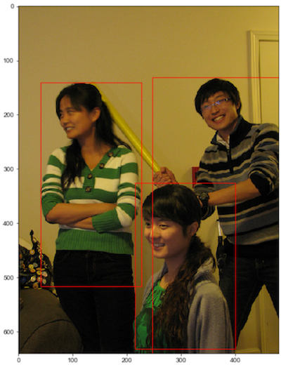
图4:边界框
通常有两种格式来表示边界框的位置:
- xyxy,即,其中是矩形框左上角的坐标,是矩形框右下角的坐标。图4中3个红色矩形框用xyxy格式表示如下:
- 左:。
- 中:。
- 右:。
- xywh,即,其中是矩形框中心点的坐标,w是矩形框的宽度,h是矩形框的高度。
在检测任务中,训练数据集的标签 里会 给出目标物体真实边界框所对应的,这样的边界框也被称为真实框(ground truth box),如 图4 所示,图中画出了3个人像所对应的真实框。模型会对目标物体可能出现的位置进行预测,由模型预测出的边界框则称为预测框(prediction box)。
注意:
- 在阅读代码时,请注意使用的是哪一种格式的 表示方式。
- 图片坐标的原点在左上角,x轴向右为正方向,y轴向下为正方向。
要完成一项检测任务,我们通常希望模型能够根据输入的图片,输出一些预测的边界框,以及边界框中所包含的物体的类别或者说属于某个类别的概率,例如这种格式: ,其中L是类别标签,P是物体属于该类别的概率。一张输入图片可能会产生多个预测框,接下来让我们一起学习如何完成这样一项任务。
锚框(Anchor box)
锚框与物体边界框不同,是由人们假想出来的一种框。先设定好锚框的大小和形状,再以图像上某一个点为中心画出矩形框。在下图中,以像素点[300, 500]为中心可以使用下面的程序生成3个框,如图中蓝色框所示,其中锚框A1跟人像区域非常接近。
# 画图展示如何绘制边界框和锚框
import numpy as np
import matplotlib.pyplot as plt
import matplotlib.patches as patches
from matplotlib.image import imread
import math

# 定义画矩形框的程序
def draw_rectangle(currentAxis, bbox, edgecolor = 'k', facecolor = 'y', fill=False, linestyle='-'):
    # currentAxis,坐标轴,通过plt.gca()获取
    # bbox,边界框,包含四个数值的list, [x1, y1, x2, y2]
    # edgecolor,边框线条颜色
    # facecolor,填充颜色
    # fill, 是否填充
    # linestype,边框线型
    # patches.Rectangle需要传入左上角坐标、矩形区域的宽度、高度等参数
    rect=patches.Rectangle((bbox[0], bbox[1]), bbox[2]-bbox[0]+1, bbox[3]-bbox[1]+1, linewidth=1,
                           edgecolor=edgecolor,facecolor=facecolor,fill=fill, linestyle=linestyle)
    currentAxis.add_patch(rect)


plt.figure(figsize=(10, 10))

filename = '/home/aistudio/work/images/section3/000000086956.jpg'
im = imread(filename)
plt.imshow(im)

# 使用xyxy格式表示物体真实框
bbox1 = [214.29, 325.03, 399.82, 631.37]
bbox2 = [40.93, 141.1, 226.99, 515.73]
bbox3 = [247.2, 131.62, 480.0, 639.32]

currentAxis=plt.gca()

draw_rectangle(currentAxis, bbox1, edgecolor='r')
draw_rectangle(currentAxis, bbox2, edgecolor='r')
draw_rectangle(currentAxis, bbox3,edgecolor='r')

# 绘制锚框
def draw_anchor_box(center, length, scales, ratios, img_height, img_width):
    """
    以center为中心,产生一系列锚框
    其中length指定了一个基准的长度
    scales是包含多种尺寸比例的list
    ratios是包含多种长宽比的list
    img_height和img_width是图片的尺寸,生成的锚框范围不能超出图片尺寸之外
    """
    bboxes = []
    for scale in scales:
        for ratio in ratios:
            h = length*scale*math.sqrt(ratio)
            w = length*scale/math.sqrt(ratio)
            x1 = max(center[0] - w/2., 0.)
            y1 = max(center[1] - h/2., 0.)
            x2 = min(center[0] + w/2. - 1.0, img_width - 1.0)
            y2 = min(center[1] + h/2. - 1.0, img_height - 1.0)
            print(center[0], center[1], w, h)
            bboxes.append([x1, y1, x2, y2])

    for bbox in bboxes:
        draw_rectangle(currentAxis, bbox, edgecolor = 'b')

img_height = im.shape[0]
img_width = im.shape[1]
draw_anchor_box([300., 500.], 100., [2.0], [0.5, 1.0, 2.0], img_height, img_width)


################# 以下为添加文字说明和箭头###############################

plt.text(285, 285, 'G1', color='red', fontsize=20)
plt.arrow(300, 288, 30, 40, color='red', width=0.001, length_includes_head=True, \
         head_width=5, head_length=10, shape='full')

plt.text(190, 320, 'A1', color='blue', fontsize=20)
plt.arrow(200, 320, 30, 40, color='blue', width=0.001, length_includes_head=True, \
         head_width=5, head_length=10, shape='full')

plt.text(160, 370, 'A2', color='blue', fontsize=20)
plt.arrow(170, 370, 30, 40, color='blue', width=0.001, length_includes_head=True, \
         head_width=5, head_length=10, shape='full')

plt.text(115, 420, 'A3', color='blue', fontsize=20)
plt.arrow(127, 420, 30, 40, color='blue', width=0.001, length_includes_head=True, \
         head_width=5, head_length=10, shape='full')

#draw_anchor_box([200., 200.], 100., [2.0], [0.5, 1.0, 2.0])
plt.show()
300.0 500.0 282.84271247461896 141.4213562373095
300.0 500.0 200.0 200.0
300.0 500.0 141.42135623730948 282.842712474619

在目标检测模型中,通常会以某种规则在图片上生成一系列锚框,将这些锚框当成可能的候选区域。模型对这些候选区域是否包含物体进行预测,如果包含目标物体,则还需要进一步预测出物体所属的类别。还有更为重要的一点是,由于锚框位置是固定的,它不大可能刚好跟物体边界框重合,所以需要在锚框的基础上进行微调以形成能准确描述物体位置的预测框,模型需要预测出微调的幅度。在训练过程中,模型通过学习不断的调整参数,最终能学会如何判别出锚框所代表的候选区域是否包含物体,如果包含物体的话,物体属于哪个类别,以及物体边界框相对于锚框位置需要调整的幅度。
不同的模型往往有着不同的生成锚框的方式,在后面的内容中,会详细介绍YOLO-V3算法里面产生锚框的规则,理解了它的设计方案,也很容易类推到其它模型上。
交并比
上面我们画出了以点为中心,生成的三个锚框,我们可以看到锚框A1 与真实框 G1的重合度比较好。那么如何衡量这三个锚框跟真实框之间的关系呢,在检测任务中是使用交并比(Intersection of Union,IoU)作为衡量指标。这一概念来源于数学中的集合,用来描述两个集合和之间的关系,它等于两个集合的交集里面所包含的元素个数,除以它们的并集里面所包含的元素个数,具体计算公式如下:
我们将用这个概念来描述两个框之间的 重合度 。两个框可以看成是两个像素的集合,它们的交并比等于两个框重合部分的面积除以它们合并起来的面积。下图“交集”中青色区域是两个框的重合面积,图“并集”中蓝色区域是两个框的相并面积。用这两个面积相除即可得到它们之间的交并比,如 图5 所示。
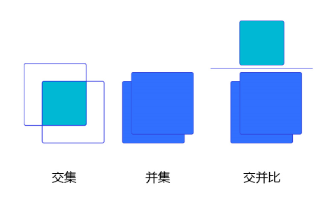
图5:交并比
假设两个矩形框A和B的位置分别为:
假如位置关系如 图6 所示:
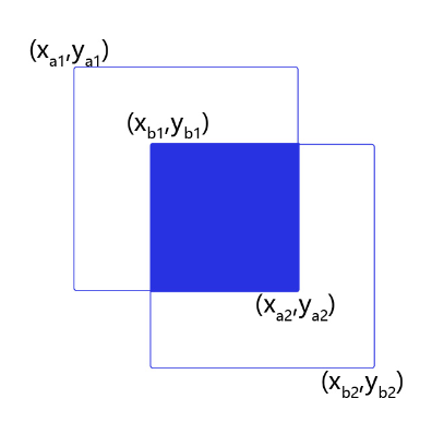
图6:计算交并比
如果二者有相交部分,则相交部分左上角坐标为:
相交部分右下角坐标为:
计算先交部分面积:
矩形框A和B的面积分别是:
计算相并部分面积:
计算交并比:
思考:
两个矩形框之间的相对位置关系,除了上面的示意图之外,还有哪些可能,上面的公式能否覆盖所有的情形?
交并比计算程序如下:
xyxy
# 计算IoU,矩形框的坐标形式为xyxy,这个函数会被保存在box_utils.py文件中
def box_iou_xyxy(box1, box2):
    # 获取box1左上角和右下角的坐标
    x1min, y1min, x1max, y1max = box1[0], box1[1], box1[2], box1[3]
    # 计算box1的面积
    s1 = (y1max - y1min + 1.) * (x1max - x1min + 1.)
    # 获取box2左上角和右下角的坐标
    x2min, y2min, x2max, y2max = box2[0], box2[1], box2[2], box2[3]
    # 计算box2的面积
    s2 = (y2max - y2min + 1.) * (x2max - x2min + 1.)

    # 计算相交矩形框的坐标
    xmin = np.maximum(x1min, x2min)
    ymin = np.maximum(y1min, y2min)
    xmax = np.minimum(x1max, x2max)
    ymax = np.minimum(y1max, y2max)
    # 计算相交矩形行的高度、宽度、面积
    inter_h = np.maximum(ymax - ymin + 1., 0.)
    inter_w = np.maximum(xmax - xmin + 1., 0.)
    intersection = inter_h * inter_w
    # 计算相并面积
    union = s1 + s2 - intersection
    # 计算交并比
    iou = intersection / union
    return iou


bbox1 = [100., 100., 200., 200.]
bbox2 = [120., 120., 220., 220.]
iou = box_iou_xyxy(bbox1, bbox2)
print('IoU is {}'.format(iou))
IoU is 0.47402644317607107
xywh
# 计算IoU,矩形框的坐标形式为xywh
def box_iou_xywh(box1, box2):
    x1min, y1min = box1[0] - box1[2]/2.0, box1[1] - box1[3]/2.0
    x1max, y1max = box1[0] + box1[2]/2.0, box1[1] + box1[3]/2.0
    s1 = box1[2] * box1[3]

    x2min, y2min = box2[0] - box2[2]/2.0, box2[1] - box2[3]/2.0
    x2max, y2max = box2[0] + box2[2]/2.0, box2[1] + box2[3]/2.0
    s2 = box2[2] * box2[3]

    xmin = np.maximum(x1min, x2min)
    ymin = np.maximum(y1min, y2min)
    xmax = np.minimum(x1max, x2max)
    ymax = np.minimum(y1max, y2max)
    inter_h = np.maximum(ymax - ymin, 0.)
    inter_w = np.maximum(xmax - xmin, 0.)
    intersection = inter_h * inter_w

    union = s1 + s2 - intersection
    iou = intersection / union
    return iou
为了直观的展示交并比的大小跟重合程度之间的关系,图7 示意了不同交并比下两个框之间的相对位置关系,从 IoU = 0.95 到 IoU = 0.
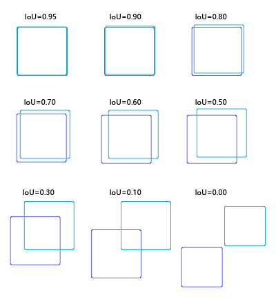
图7:不同交并比下两个框之间相对位置示意图
问题:
- 什么情况下两个矩形框的IoU等于1?
- 什么情况下两个矩形框的IoU等于0?
林业病虫害数据集和数据预处理方法介绍
在本次的课程中,将使用百度与林业大学合作开发的林业病虫害防治项目中用到昆虫数据集,关于该项目和数据集的更多信息,可以参考相关报道。在这一小节中将为读者介绍该数据集,以及计算机视觉任务中常用的数据预处理方法。
读取AI识虫数据集标注信息
AI识虫数据集结构如下:
- 提供了2183张图片,其中训练集1693张,验证集245,测试集245张。
- 包含7种昆虫,分别是Boerner、Leconte、Linnaeus、acuminatus、armandi、coleoptera和linnaeus。
- 包含了图片和标注,请读者先将数据解压,并存放在insects目录下。
# 解压数据脚本,第一次运行时打开注释,将文件解压到work目录下
!unzip -d /home/aistudio/work /home/aistudio/data/data19638/insects.zip
将数据解压之后,可以看到insects目录下的结构如下所示。
    insects
        |---train
        |         |---annotations
        |         |         |---xmls
        |         |                  |---100.xml
        |         |                  |---101.xml
        |         |                  |---...
        |         |
        |         |---images
        |                   |---100.jpeg
        |                   |---101.jpeg
        |                   |---...
        |
        |---val
        |        |---annotations
        |        |         |---xmls
        |        |                  |---1221.xml
        |        |                  |---1277.xml
        |        |                  |---...
        |        |
        |        |---images
        |                  |---1221.jpeg
        |                  |---1277.jpeg
        |                  |---...
        |
        |---test
                 |---images
                           |---1833.jpeg
                           |---1838.jpeg
                           |---...
insects包含train、val和test三个文件夹。train/annotations/xmls目录下存放着图片的标注。每个xml文件是对一张图片的说明,包括图片尺寸、包含的昆虫名称、在图片上出现的位置等信息。
<annotation>
        <folder>刘霏霏</folder>
        <filename>100.jpeg</filename>
        <path>/home/fion/桌面/刘霏霏/100.jpeg</path>
        <source>
                <database>Unknown</database>
        </source>
        <size>
                <width>1336</width>
                <height>1336</height>
                <depth>3</depth>
        </size>
        <segmented>0</segmented>
        <object>
                <name>Boerner</name>
                <pose>Unspecified</pose>
                <truncated>0</truncated>
                <difficult>0</difficult>
                <bndbox>
                        <xmin>500</xmin>
                        <ymin>893</ymin>
                        <xmax>656</xmax>
                        <ymax>966</ymax>
                </bndbox>
        </object>
        <object>
                <name>Leconte</name>
                <pose>Unspecified</pose>
                <truncated>0</truncated>
                <difficult>0</difficult>
                <bndbox>
                        <xmin>622</xmin>
                        <ymin>490</ymin>
                        <xmax>756</xmax>
                        <ymax>610</ymax>
                </bndbox>
        </object>
        <object>
                <name>armandi</name>
                <pose>Unspecified</pose>
                <truncated>0</truncated>
                <difficult>0</difficult>
                <bndbox>
                        <xmin>432</xmin>
                        <ymin>663</ymin>
                        <xmax>517</xmax>
                        <ymax>729</ymax>
                </bndbox>
        </object>
        <object>
                <name>coleoptera</name>
                <pose>Unspecified</pose>
                <truncated>0</truncated>
                <difficult>0</difficult>
                <bndbox>
                        <xmin>624</xmin>
                        <ymin>685</ymin>
                        <xmax>697</xmax>
                        <ymax>771</ymax>
                </bndbox>
        </object>
        <object>
                <name>linnaeus</name>
                <pose>Unspecified</pose>
                <truncated>0</truncated>
                <difficult>0</difficult>
                <bndbox>
                        <xmin>783</xmin>
                        <ymin>700</ymin>
                        <xmax>856</xmax>
                        <ymax>802</ymax>
                </bndbox>
        </object>
</annotation>
上面列出的xml文件中的主要参数说明如下:
size:图片尺寸
object:图片中包含的物体,一张图片可能中包含多个物体
- name:昆虫名称
- bndbox:物体真实框
- difficult:识别是否困难
下面我们将从数据集中读取xml文件,将每张图片的标注信息读取出来。在读取具体的标注文件之前,我们先完成一件事情,就是将昆虫的类别名字(字符串)转化成数字表示的类别。因为神经网络里面计算时需要的输入类型是数值型的,所以需要将字符串表示的类别转化成具体的数字。昆虫类别名称的列表是:[‘Boerner’, ‘Leconte’, ‘Linnaeus’, ‘acuminatus’, ‘armandi’, ‘coleoptera’, ‘linnaeus’],这里我们约定此列表中:'Boerner’对应类别0,'Leconte’对应类别1,…,'linnaeus’对应类别6。使用下面的程序可以得到表示名称字符串和数字类别之间映射关系的字典。
INSECT_NAMES = ['Boerner', 'Leconte', 'Linnaeus',
                'acuminatus', 'armandi', 'coleoptera', 'linnaeus']

def get_insect_names():
    """
    return a dict, as following,
        {'Boerner': 0,
         'Leconte': 1,
         'Linnaeus': 2,
         'acuminatus': 3,
         'armandi': 4,
         'coleoptera': 5,
         'linnaeus': 6
        }
    It can map the insect name into an integer label.
    """
    insect_category2id = {}
    for i, item in enumerate(INSECT_NAMES):
        insect_category2id[item] = i

    return insect_category2id
cname2cid = get_insect_names()
cname2cid
{'Boerner': 0,
 'Leconte': 1,
 'Linnaeus': 2,
 'acuminatus': 3,
 'armandi': 4,
 'coleoptera': 5,
 'linnaeus': 6}
调用get_insect_names函数返回一个dict,其键-值对描述了昆虫名称-数字类别之间的映射关系。
下面的程序从annotations/xml目录下面读取所有文件标注信息。
import os
import numpy as np
import xml.etree.ElementTree as ET

def get_annotations(cname2cid, datadir):
    filenames = os.listdir(os.path.join(datadir, 'annotations', 'xmls'))
    records = []
    ct = 0
    for fname in filenames:
        fid = fname.split('.')[0]
        fpath = os.path.join(datadir, 'annotations', 'xmls', fname)
        img_file = os.path.join(datadir, 'images', fid + '.jpeg')
        tree = ET.parse(fpath)

        if tree.find('id') is None:
            im_id = np.array([ct])
        else:
            im_id = np.array([int(tree.find('id').text)])

        objs = tree.findall('object')
        im_w = float(tree.find('size').find('width').text)
        im_h = float(tree.find('size').find('height').text)
        gt_bbox = np.zeros((len(objs), 4), dtype=np.float32)
        gt_class = np.zeros((len(objs), ), dtype=np.int32)
        is_crowd = np.zeros((len(objs), ), dtype=np.int32)
        difficult = np.zeros((len(objs), ), dtype=np.int32)
        for i, obj in enumerate(objs):
            cname = obj.find('name').text
            gt_class[i] = cname2cid[cname]
            _difficult = int(obj.find('difficult').text)
            x1 = float(obj.find('bndbox').find('xmin').text)
            y1 = float(obj.find('bndbox').find('ymin').text)
            x2 = float(obj.find('bndbox').find('xmax').text)
            y2 = float(obj.find('bndbox').find('ymax').text)
            x1 = max(0, x1)
            y1 = max(0, y1)
            x2 = min(im_w - 1, x2)
            y2 = min(im_h - 1, y2)
            # 这里使用xywh格式来表示目标物体真实框
            gt_bbox[i] = [(x1+x2)/2.0 , (y1+y2)/2.0, x2-x1+1., y2-y1+1.]
            is_crowd[i] = 0
            difficult[i] = _difficult

        voc_rec = {
            'im_file': img_file,
            'im_id': im_id,
            'h': im_h,
            'w': im_w,
            'is_crowd': is_crowd,
            'gt_class': gt_class,
            'gt_bbox': gt_bbox,
            'gt_poly': [],
            'difficult': difficult
            }
        if len(objs) != 0:
            records.append(voc_rec)
        ct += 1
    return records
TRAINDIR = '/home/aistudio/work/insects/train'
TESTDIR = '/home/aistudio/work/insects/test'
VALIDDIR = '/home/aistudio/work/insects/val'
cname2cid = get_insect_names()
records = get_annotations(cname2cid, TRAINDIR)
len(records)
1693
records[0]
{'im_file': '/home/aistudio/work/insects/train/images/2140.jpeg',
 'im_id': array([0]),
 'h': 1222.0,
 'w': 1222.0,
 'is_crowd': array([0, 0, 0, 0, 0, 0, 0, 0], dtype=int32),
 'gt_class': array([1, 1, 1, 2, 4, 3, 5, 0], dtype=int32),
 'gt_bbox': array([[603. , 382. , 129. , 131. ],
        [853. , 764.5, 131. , 116. ],
        [531.5, 849. , 138. , 121. ],
        [721. , 890. ,  63. ,  85. ],
        [604.5, 613. ,  70. ,  85. ],
        [814. , 471.5,  47. ,  86. ],
        [752.5, 610.5,  62. ,  38. ],
        [570. , 771.5,  79. , 116. ]], dtype=float32),
 'gt_poly': [],
 'difficult': array([0, 0, 0, 0, 0, 0, 0, 0], dtype=int32)}
通过上面的程序,将所有训练数据集的标注数据全部读取出来了,存放在records列表下面,其中每一个元素是一张图片的标注数据,包含了图片存放地址,图片id,图片高度和宽度,图片中所包含的目标物体的种类和位置。
数据读取和预处理
数据预处理是训练神经网络时非常重要的步骤。合适的预处理方法,可以帮助模型更好的收敛并防止过拟合。首先我们需要从磁盘读入数据,然后需要对这些数据进行预处理,为了保证网络运行的速度通常还要对数据预处理进行加速。
数据读取
前面已经将图片的所有描述信息保存在records中了,其中的每一个元素包含了一张图片的描述,下面的程序展示了如何根据records里面的描述读取图片及标注。
### 数据读取
import cv2

def get_bbox(gt_bbox, gt_class):
    # 对于一般的检测任务来说,一张图片上往往会有多个目标物体
    # 设置参数MAX_NUM = 50, 即一张图片最多取50个真实框;如果真实
    # 框的数目少于50个,则将不足部分的gt_bbox, gt_class和gt_score的各项数值全设置为0
    MAX_NUM = 50
    gt_bbox2 = np.zeros((MAX_NUM, 4))
    gt_class2 = np.zeros((MAX_NUM,))
    for i in range(len(gt_bbox)):
        gt_bbox2[i, :] = gt_bbox[i, :]
        gt_class2[i] = gt_class[i]
        if i >= MAX_NUM:
            break
    return gt_bbox2, gt_class2

def get_img_data_from_file(record):
    """
    record is a dict as following,
      record = {
            'im_file': img_file,
            'im_id': im_id,
            'h': im_h,
            'w': im_w,
            'is_crowd': is_crowd,
            'gt_class': gt_class,
            'gt_bbox': gt_bbox,
            'gt_poly': [],
            'difficult': difficult
            }
    """
    im_file = record['im_file']
    h = record['h']
    w = record['w']
    is_crowd = record['is_crowd']
    gt_class = record['gt_class']
    gt_bbox = record['gt_bbox']
    difficult = record['difficult']

    img = cv2.imread(im_file)
    img = cv2.cvtColor(img, cv2.COLOR_BGR2RGB)

    # check if h and w in record equals that read from img
    assert img.shape[0] == int(h), \
             "image height of {} inconsistent in record({}) and img file({})".format(
               im_file, h, img.shape[0])

    assert img.shape[1] == int(w), \
             "image width of {} inconsistent in record({}) and img file({})".format(
               im_file, w, img.shape[1])

    gt_boxes, gt_labels = get_bbox(gt_bbox, gt_class)

    # gt_bbox 用相对值
    gt_boxes[:, 0] = gt_boxes[:, 0] / float(w)
    gt_boxes[:, 1] = gt_boxes[:, 1] / float(h)
    gt_boxes[:, 2] = gt_boxes[:, 2] / float(w)
    gt_boxes[:, 3] = gt_boxes[:, 3] / float(h)

    return img, gt_boxes, gt_labels, (h, w)
record = records[0]
img, gt_boxes, gt_labels, scales = get_img_data_from_file(record)
img.shape
(1222, 1222, 3)
gt_boxes.shape
(50, 4)
gt_labels
array([1., 1., 0., 2., 3., 4., 5., 5., 0., 0., 0., 0., 0., 0., 0., 0., 0.,
       0., 0., 0., 0., 0., 0., 0., 0., 0., 0., 0., 0., 0., 0., 0., 0., 0.,
       0., 0., 0., 0., 0., 0., 0., 0., 0., 0., 0., 0., 0., 0., 0., 0.])
scales
(1222.0, 1222.0)
get_img_data_from_file()函数可以返回图片数据的数据,它们是图像数据img, 真实框坐标gt_boxes, 真实框包含的物体类别gt_labels, 图像尺寸scales。
数据预处理
在计算机视觉中,通常会对图像做一些随机的变化,产生相似但又不完全相同的样本。主要作用是扩大训练数据集,抑制过拟合,提升模型的泛化能力,常用的方法见下面的程序。
随机改变亮暗、对比度和颜色等
import numpy as np
import cv2
from PIL import Image, ImageEnhance
import random

# 随机改变亮暗、对比度和颜色等
def random_distort(img):
    # 随机改变亮度
    def random_brightness(img, lower=0.5, upper=1.5):
        e = np.random.uniform(lower, upper)
        return ImageEnhance.Brightness(img).enhance(e)
    # 随机改变对比度
    def random_contrast(img, lower=0.5, upper=1.5):
        e = np.random.uniform(lower, upper)
        return ImageEnhance.Contrast(img).enhance(e)
    # 随机改变颜色
    def random_color(img, lower=0.5, upper=1.5):
        e = np.random.uniform(lower, upper)
        return ImageEnhance.Color(img).enhance(e)

    ops = [random_brightness, random_contrast, random_color]
    np.random.shuffle(ops)

    img = Image.fromarray(img)
    img = ops[0](img)
    img = ops[1](img)
    img = ops[2](img)
    img = np.asarray(img)

    return img
随机填充
# 随机填充
def random_expand(img,
                  gtboxes,
                  max_ratio=4.,
                  fill=None,
                  keep_ratio=True,
                  thresh=0.5):
    if random.random() > thresh:
        return img, gtboxes

    if max_ratio < 1.0:
        return img, gtboxes

    h, w, c = img.shape
    ratio_x = random.uniform(1, max_ratio)
    if keep_ratio:
        ratio_y = ratio_x
    else:
        ratio_y = random.uniform(1, max_ratio)
    oh = int(h * ratio_y)
    ow = int(w * ratio_x)
    off_x = random.randint(0, ow - w)
    off_y = random.randint(0, oh - h)

    out_img = np.zeros((oh, ow, c))
    if fill and len(fill) == c:
        for i in range(c):
            out_img[:, :, i] = fill[i] * 255.0

    out_img[off_y:off_y + h, off_x:off_x + w, :] = img
    gtboxes[:, 0] = ((gtboxes[:, 0] * w) + off_x) / float(ow)
    gtboxes[:, 1] = ((gtboxes[:, 1] * h) + off_y) / float(oh)
    gtboxes[:, 2] = gtboxes[:, 2] / ratio_x
    gtboxes[:, 3] = gtboxes[:, 3] / ratio_y

    return out_img.astype('uint8'), gtboxes
随机裁剪
随机裁剪之前需要先定义两个函数,multi_box_iou_xywh和box_crop这两个函数将被保存在box_utils.py文件中。
import numpy as np

def multi_box_iou_xywh(box1, box2):
    """
    In this case, box1 or box2 can contain multi boxes.
    Only two cases can be processed in this method:
       1, box1 and box2 have the same shape, box1.shape == box2.shape
       2, either box1 or box2 contains only one box, len(box1) == 1 or len(box2) == 1
    If the shape of box1 and box2 does not match, and both of them contain multi boxes, it will be wrong.
    """
    assert box1.shape[-1] == 4, "Box1 shape[-1] should be 4."
    assert box2.shape[-1] == 4, "Box2 shape[-1] should be 4."


    b1_x1, b1_x2 = box1[:, 0] - box1[:, 2] / 2, box1[:, 0] + box1[:, 2] / 2
    b1_y1, b1_y2 = box1[:, 1] - box1[:, 3] / 2, box1[:, 1] + box1[:, 3] / 2
    b2_x1, b2_x2 = box2[:, 0] - box2[:, 2] / 2, box2[:, 0] + box2[:, 2] / 2
    b2_y1, b2_y2 = box2[:, 1] - box2[:, 3] / 2, box2[:, 1] + box2[:, 3] / 2

    inter_x1 = np.maximum(b1_x1, b2_x1)
    inter_x2 = np.minimum(b1_x2, b2_x2)
    inter_y1 = np.maximum(b1_y1, b2_y1)
    inter_y2 = np.minimum(b1_y2, b2_y2)
    inter_w = inter_x2 - inter_x1
    inter_h = inter_y2 - inter_y1
    inter_w = np.clip(inter_w, a_min=0., a_max=None)
    inter_h = np.clip(inter_h, a_min=0., a_max=None)

    inter_area = inter_w * inter_h
    b1_area = (b1_x2 - b1_x1) * (b1_y2 - b1_y1)
    b2_area = (b2_x2 - b2_x1) * (b2_y2 - b2_y1)

    return inter_area / (b1_area + b2_area - inter_area)

def box_crop(boxes, labels, crop, img_shape):
    x, y, w, h = map(float, crop)
    im_w, im_h = map(float, img_shape)

    boxes = boxes.copy()
    boxes[:, 0], boxes[:, 2] = (boxes[:, 0] - boxes[:, 2] / 2) * im_w, (
        boxes[:, 0] + boxes[:, 2] / 2) * im_w
    boxes[:, 1], boxes[:, 3] = (boxes[:, 1] - boxes[:, 3] / 2) * im_h, (
        boxes[:, 1] + boxes[:, 3] / 2) * im_h

    crop_box = np.array([x, y, x + w, y + h])
    centers = (boxes[:, :2] + boxes[:, 2:]) / 2.0
    mask = np.logical_and(crop_box[:2] <= centers, centers <= crop_box[2:]).all(
        axis=1)

    boxes[:, :2] = np.maximum(boxes[:, :2], crop_box[:2])
    boxes[:, 2:] = np.minimum(boxes[:, 2:], crop_box[2:])
    boxes[:, :2] -= crop_box[:2]
    boxes[:, 2:] -= crop_box[:2]

    mask = np.logical_and(mask, (boxes[:, :2] < boxes[:, 2:]).all(axis=1))
    boxes = boxes * np.expand_dims(mask.astype('float32'), axis=1)
    labels = labels * mask.astype('float32')
    boxes[:, 0], boxes[:, 2] = (boxes[:, 0] + boxes[:, 2]) / 2 / w, (
        boxes[:, 2] - boxes[:, 0]) / w
    boxes[:, 1], boxes[:, 3] = (boxes[:, 1] + boxes[:, 3]) / 2 / h, (
        boxes[:, 3] - boxes[:, 1]) / h

    return boxes, labels, mask.sum()
# 随机裁剪
def random_crop(img,
                boxes,
                labels,
                scales=[0.3, 1.0],
                max_ratio=2.0,
                constraints=None,
                max_trial=50):
    if len(boxes) == 0:
        return img, boxes

    if not constraints:
        constraints = [(0.1, 1.0), (0.3, 1.0), (0.5, 1.0), (0.7, 1.0),
                       (0.9, 1.0), (0.0, 1.0)]

    img = Image.fromarray(img)
    w, h = img.size
    crops = [(0, 0, w, h)]
    for min_iou, max_iou in constraints:
        for _ in range(max_trial):
            scale = random.uniform(scales[0], scales[1])
            aspect_ratio = random.uniform(max(1 / max_ratio, scale * scale), \
                                          min(max_ratio, 1 / scale / scale))
            crop_h = int(h * scale / np.sqrt(aspect_ratio))
            crop_w = int(w * scale * np.sqrt(aspect_ratio))
            crop_x = random.randrange(w - crop_w)
            crop_y = random.randrange(h - crop_h)
            crop_box = np.array([[(crop_x + crop_w / 2.0) / w,
                                  (crop_y + crop_h / 2.0) / h,
                                  crop_w / float(w), crop_h / float(h)]])

            iou = multi_box_iou_xywh(crop_box, boxes)
            if min_iou <= iou.min() and max_iou >= iou.max():
                crops.append((crop_x, crop_y, crop_w, crop_h))
                break

    while crops:
        crop = crops.pop(np.random.randint(0, len(crops)))
        crop_boxes, crop_labels, box_num = box_crop(boxes, labels, crop, (w, h))
        if box_num < 1:
            continue
        img = img.crop((crop[0], crop[1], crop[0] + crop[2],
                        crop[1] + crop[3])).resize(img.size, Image.LANCZOS)
        img = np.asarray(img)
        return img, crop_boxes, crop_labels
    img = np.asarray(img)
    return img, boxes, labels
随机缩放
# 随机缩放
def random_interp(img, size, interp=None):
    interp_method = [
        cv2.INTER_NEAREST,
        cv2.INTER_LINEAR,
        cv2.INTER_AREA,
        cv2.INTER_CUBIC,
        cv2.INTER_LANCZOS4,
    ]
    if not interp or interp not in interp_method:
        interp = interp_method[random.randint(0, len(interp_method) - 1)]
    h, w, _ = img.shape
    im_scale_x = size / float(w)
    im_scale_y = size / float(h)
    img = cv2.resize(
        img, None, None, fx=im_scale_x, fy=im_scale_y, interpolation=interp)
    return img
随机翻转
# 随机翻转
def random_flip(img, gtboxes, thresh=0.5):
    if random.random() > thresh:
        img = img[:, ::-1, :]
        gtboxes[:, 0] = 1.0 - gtboxes[:, 0]
    return img, gtboxes
随机打乱真实框排列顺序
# 随机打乱真实框排列顺序
def shuffle_gtbox(gtbox, gtlabel):
    gt = np.concatenate(
        [gtbox, gtlabel[:, np.newaxis]], axis=1)
    idx = np.arange(gt.shape[0])
    np.random.shuffle(idx)
    gt = gt[idx, :]
    return gt[:, :4], gt[:, 4]
图像增广方法
# 图像增广方法汇总
def image_augment(img, gtboxes, gtlabels, size, means=None):
    # 随机改变亮暗、对比度和颜色等
    img = random_distort(img)
    # 随机填充
    img, gtboxes = random_expand(img, gtboxes, fill=means)
    # 随机裁剪
    img, gtboxes, gtlabels, = random_crop(img, gtboxes, gtlabels)
    # 随机缩放
    img = random_interp(img, size)
    # 随机翻转
    img, gtboxes = random_flip(img, gtboxes)
    # 随机打乱真实框排列顺序
    gtboxes, gtlabels = shuffle_gtbox(gtboxes, gtlabels)

    return img.astype('float32'), gtboxes.astype('float32'), gtlabels.astype('int32')
img, gt_boxes, gt_labels, scales = get_img_data_from_file(record)
size = 512
img, gt_boxes, gt_labels = image_augment(img, gt_boxes, gt_labels, size)
img.shape
(512, 512, 3)
gt_boxes.shape
(50, 4)
gt_labels.shape
(50,)
这里得到的img数据数值需要调整,需要除以255,并且减去均值和方差,再将维度从[H, W, C]调整为[C, H, W]
img, gt_boxes, gt_labels, scales = get_img_data_from_file(record)
size = 512
img, gt_boxes, gt_labels = image_augment(img, gt_boxes, gt_labels, size)
mean = [0.485, 0.456, 0.406]
std = [0.229, 0.224, 0.225]
mean = np.array(mean).reshape((1, 1, -1))
std = np.array(std).reshape((1, 1, -1))
img = (img / 255.0 - mean) / std
img = img.astype('float32').transpose((2, 0, 1))
img
array([[[-2.117904 , -2.117904 , -2.117904 , ..., -2.117904 ,
         -2.117904 , -2.117904 ],
        [-2.117904 , -2.117904 , -2.117904 , ..., -2.117904 ,
         -2.117904 , -2.117904 ],
        [-2.117904 , -2.117904 , -2.117904 , ..., -2.117904 ,
         -2.117904 , -2.117904 ],
        ...,
        [-2.117904 , -2.117904 , -2.117904 , ..., -2.117904 ,
         -2.117904 , -2.117904 ],
        [-2.117904 , -2.117904 , -2.117904 , ..., -2.117904 ,
         -2.117904 , -2.117904 ],
        [-2.117904 , -2.117904 , -2.117904 , ..., -2.117904 ,
         -2.117904 , -2.117904 ]],

       [[-2.0357144, -2.0357144, -2.0357144, ..., -2.0357144,
         -2.0357144, -2.0357144],
        [-2.0357144, -2.0357144, -2.0357144, ..., -2.0357144,
         -2.0357144, -2.0357144],
        [-2.0357144, -2.0357144, -2.0357144, ..., -2.0357144,
         -2.0357144, -2.0357144],
        ...,
        [-2.0357144, -2.0357144, -2.0357144, ..., -2.0357144,
         -2.0357144, -2.0357144],
        [-2.0357144, -2.0357144, -2.0357144, ..., -2.0357144,
         -2.0357144, -2.0357144],
        [-2.0357144, -2.0357144, -2.0357144, ..., -2.0357144,
         -2.0357144, -2.0357144]],

       [[-1.8044444, -1.8044444, -1.8044444, ..., -1.8044444,
         -1.8044444, -1.8044444],
        [-1.8044444, -1.8044444, -1.8044444, ..., -1.8044444,
         -1.8044444, -1.8044444],
        [-1.8044444, -1.8044444, -1.8044444, ..., -1.8044444,
         -1.8044444, -1.8044444],
        ...,
        [-1.8044444, -1.8044444, -1.8044444, ..., -1.8044444,
         -1.8044444, -1.8044444],
        [-1.8044444, -1.8044444, -1.8044444, ..., -1.8044444,
         -1.8044444, -1.8044444],
        [-1.8044444, -1.8044444, -1.8044444, ..., -1.8044444,
         -1.8044444, -1.8044444]]], dtype=float32)
将上面的过程整理成一个函数get_img_data
def get_img_data(record, size=640):
    img, gt_boxes, gt_labels, scales = get_img_data_from_file(record)
    img, gt_boxes, gt_labels = image_augment(img, gt_boxes, gt_labels, size)
    mean = [0.485, 0.456, 0.406]
    std = [0.229, 0.224, 0.225]
    mean = np.array(mean).reshape((1, 1, -1))
    std = np.array(std).reshape((1, 1, -1))
    img = (img / 255.0 - mean) / std
    img = img.astype('float32').transpose((2, 0, 1))
    return img, gt_boxes, gt_labels, scales
TRAINDIR = '/home/aistudio/work/insects/train'
TESTDIR = '/home/aistudio/work/insects/test'
VALIDDIR = '/home/aistudio/work/insects/val'
cname2cid = get_insect_names()
records = get_annotations(cname2cid, TRAINDIR)

record = records[0]
img, gt_boxes, gt_labels, scales = get_img_data(record, size=480)
img.shape
(3, 480, 480)
gt_boxes.shape
(50, 4)
gt_labels
array([0, 0, 0, 0, 0, 0, 0, 0, 0, 0, 0, 0, 0, 0, 0, 0, 0, 0, 0, 0, 0, 0,
       0, 0, 0, 0, 0, 0, 0, 0, 0, 0, 0, 0, 0, 0, 0, 0, 0, 0, 1, 0, 0, 0,
       0, 4, 0, 0, 0, 0], dtype=int32)
scales
(1244.0, 1244.0)
批量数据读取与加速
上面的程序展示了如何读取一张图片的数据并加速,下面的代码实现了批量数据读取。
# 获取一个批次内样本随机缩放的尺寸
def get_img_size(mode):
    if (mode == 'train') or (mode == 'valid'):
        inds = np.array([0,1,2,3,4,5,6,7,8,9])
        ii = np.random.choice(inds)
        img_size = 320 + ii * 32
    else:
        img_size = 608
    return img_size

# 将 list形式的batch数据 转化成多个array构成的tuple
def make_array(batch_data):
    img_array = np.array([item[0] for item in batch_data], dtype = 'float32')
    gt_box_array = np.array([item[1] for item in batch_data], dtype = 'float32')
    gt_labels_array = np.array([item[2] for item in batch_data], dtype = 'int32')
    img_scale = np.array([item[3] for item in batch_data], dtype='int32')
    return img_array, gt_box_array, gt_labels_array, img_scale

# 批量读取数据,同一批次内图像的尺寸大小必须是一样的,
# 不同批次之间的大小是随机的,
# 由上面定义的get_img_size函数产生
def data_loader(datadir, batch_size= 10, mode='train'):
    cname2cid = get_insect_names()
    records = get_annotations(cname2cid, datadir)

    def reader():
        if mode == 'train':
            np.random.shuffle(records)
        batch_data = []
        img_size = get_img_size(mode)
        for record in records:
            #print(record)
            img, gt_bbox, gt_labels, im_shape = get_img_data(record,
                                                             size=img_size)
            batch_data.append((img, gt_bbox, gt_labels, im_shape))
            if len(batch_data) == batch_size:
                yield make_array(batch_data)
                batch_data = []
                img_size = get_img_size(mode)
        if len(batch_data) > 0:
            yield make_array(batch_data)

    return reader
d = data_loader('/home/aistudio/work/insects/train', batch_size=2, mode='train')
img, gt_boxes, gt_labels, im_shape = next(d())
img.shape, gt_boxes.shape, gt_labels.shape, im_shape.shape
((2, 3, 352, 352), (2, 50, 4), (2, 50), (2, 2))
由于数据预处理耗时较长,可能会成为网络训练速度的瓶颈,所以需要对预处理部分进行优化。通过使用飞桨提供的API paddle.reader.xmap_readers可以开启多线程读取数据,具体实现代码如下。
import functools
import paddle

# 使用paddle.reader.xmap_readers实现多线程读取数据
def multithread_loader(datadir, batch_size= 10, mode='train'):
    cname2cid = get_insect_names()
    records = get_annotations(cname2cid, datadir)
    def reader():
        if mode == 'train':
            np.random.shuffle(records)
        img_size = get_img_size(mode)
        batch_data = []
        for record in records:
            batch_data.append((record, img_size))
            if len(batch_data) == batch_size:
                yield batch_data
                batch_data = []
                img_size = get_img_size(mode)
        if len(batch_data) > 0:
            yield batch_data

    def get_data(samples):
        batch_data = []
        for sample in samples:
            record = sample[0]
            img_size = sample[1]
            img, gt_bbox, gt_labels, im_shape = get_img_data(record, size=img_size)
            batch_data.append((img, gt_bbox, gt_labels, im_shape))
        return make_array(batch_data)

    mapper = functools.partial(get_data, )

    return paddle.reader.xmap_readers(mapper, reader, 8, 10)
d = multithread_loader('/home/aistudio/work/insects/train', batch_size=2, mode='train')
img, gt_boxes, gt_labels, im_shape = next(d())
img.shape, gt_boxes.shape, gt_labels.shape, im_shape.shape
((2, 3, 416, 416), (2, 50, 4), (2, 50), (2, 2))
至此,我们完成了 如何查看数据集中的数据、提取数据标注信息、从文件读取图像和标注数据、图像增广、批量读取和加速等过程,通过multithread_loader可以返回img, gt_boxes, gt_labels, im_shape等数据,接下来就可以将它们输入到神经网络,应用到具体算法上了。
在开始具体的算法讲解之前,先补充一下读取测试数据的代码。测试数据没有标注信息,也不需要做图像增广,代码如下所示。
# 测试数据读取

# 将 list形式的batch数据 转化成多个array构成的tuple
def make_test_array(batch_data):
    img_name_array = np.array([item[0] for item in batch_data])
    img_data_array = np.array([item[1] for item in batch_data], dtype = 'float32')
    img_scale_array = np.array([item[2] for item in batch_data], dtype='int32')
    return img_name_array, img_data_array, img_scale_array

# 测试数据读取
def test_data_loader(datadir, batch_size= 10, test_image_size=608, mode='test'):
    """
    加载测试用的图片,测试数据没有groundtruth标签
    """
    image_names = os.listdir(datadir)
    def reader():
        batch_data = []
        img_size = test_image_size
        for image_name in image_names:
            file_path = os.path.join(datadir, image_name)
            img = cv2.imread(file_path)
            img = cv2.cvtColor(img, cv2.COLOR_BGR2RGB)
            H = img.shape[0]
            W = img.shape[1]
            img = cv2.resize(img, (img_size, img_size))

            mean = [0.485, 0.456, 0.406]
            std = [0.229, 0.224, 0.225]
            mean = np.array(mean).reshape((1, 1, -1))
            std = np.array(std).reshape((1, 1, -1))
            out_img = (img / 255.0 - mean) / std
            out_img = out_img.astype('float32').transpose((2, 0, 1))
            img = out_img #np.transpose(out_img, (2,0,1))
            im_shape = [H, W]

            batch_data.append((image_name.split('.')[0], img, im_shape))
            if len(batch_data) == batch_size:
                yield make_test_array(batch_data)
                batch_data = []
        if len(batch_data) > 0:
            yield make_test_array(batch_data)

    return reader
