

使用sktime预测
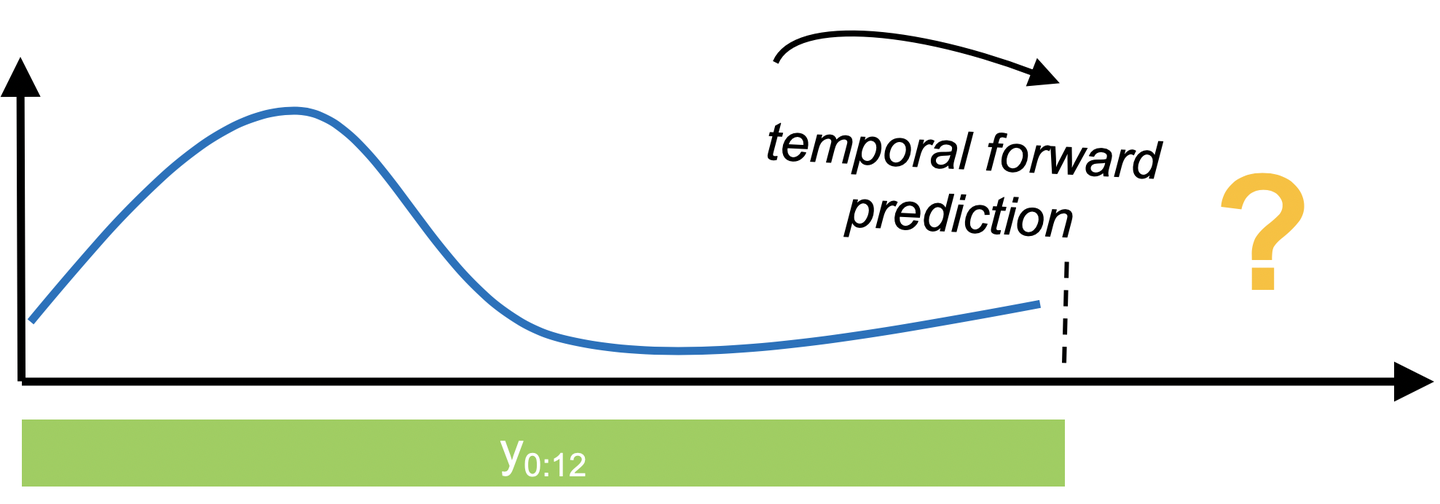
在预测中,我们对利用过去的数据进行对未来进行预测很感兴趣。sktime提供了常用的统计预测算法和用于建立复合机器学习模型的工具。
更多细节,请看我们关于用sktime进行预测的论文,其中我们更详细地讨论了 forecasting API,并使用它来复制和扩展M4研究。
准备工作
[2]:
from warnings import simplefilter

import numpy as np
import pandas as pd

from sktime.datasets import load_airline
from sktime.forecasting.arima import ARIMA, AutoARIMA
from sktime.forecasting.base import ForecastingHorizon
from sktime.forecasting.compose import (
    EnsembleForecaster,
    ReducedRegressionForecaster,
    TransformedTargetForecaster,
)
from sktime.forecasting.exp_smoothing import ExponentialSmoothing
from sktime.forecasting.model_selection import (
    ForecastingGridSearchCV,
    SlidingWindowSplitter,
    temporal_train_test_split,
)
from sktime.forecasting.naive import NaiveForecaster
from sktime.forecasting.theta import ThetaForecaster
from sktime.forecasting.trend import PolynomialTrendForecaster
from sktime.performance_metrics.forecasting import sMAPE, smape_loss
from sktime.transformations.series.detrend import Deseasonalizer, Detrender
from sktime.utils.plotting import plot_series

simplefilter("ignore", FutureWarning)
%matplotlib inline
数据
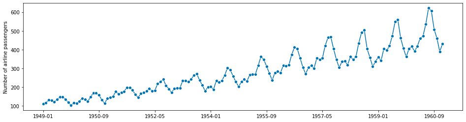
首先,我们使用Box-Jenkins单变量航空数据集,该数据集显示了1949-1960年每月的国际航空乘客数量。
[3]:
y = load_airline()
plot_series(y);
一个时间序列由一系列时间点-数值对组成,其中数值代表我们观察到的数值,时间点代表我们观察到该数值的时间点。
我们将时间序列表示为pd.Series,其中索引代表时间点。sktime支持pandas的integer, period 和timestamp。在这个例子中,我们有一个period index。
[4]:
y.index
[4]:
PeriodIndex(['1949-01', '1949-02', '1949-03', '1949-04', '1949-05', '1949-06',
             '1949-07', '1949-08', '1949-09', '1949-10',
             ...
             '1960-03', '1960-04', '1960-05', '1960-06', '1960-07', '1960-08',
             '1960-09', '1960-10', '1960-11', '1960-12'],
            dtype='period[M]', name='Period', length=144, freq='M')
明确预测任务
接下来我们将定义一个预测任务。
- 我们将尝试预测最近3年的数据,使用前几年的数据作为训练数据。系列中的每一个点代表一个月,所以我们应该保留最后36个点作为测试数据,并使用36步的超前预测范围来评估预测性能。
- 我们将使用sMAPE(对称平均绝对误差百分比)来量化我们预测的准确性。较低的sMAPE意味着较高的准确性。
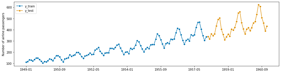
我们可以对数据进行如下拆分。
[5]:
y_train, y_test = temporal_train_test_split(y, test_size=36)
plot_series(y_train, y_test, labels=["y_train", "y_test"])
print(y_train.shape[0], y_test.shape[0])
108 36
当我们进行预测时,我们需要指定预测范围,并将其传递给我们的预测算法。
相对预测范围
One of the simplest ways is to define a np.array with the steps ahead that you want to predict relative to the end of the training series.
(这句不知咋翻译好)
[6]:
fh = np.arange(len(y_test)) + 1
fh
[6]:
array([ 1,  2,  3,  4,  5,  6,  7,  8,  9, 10, 11, 12, 13, 14, 15, 16, 17,
       18, 19, 20, 21, 22, 23, 24, 25, 26, 27, 28, 29, 30, 31, 32, 33, 34,
       35, 36])
所以这里我们感兴趣的是从第一步到第三十六步的预测。当然你也可以你使用其他的预测范围。例如,如果只预测前面的第二步和第五步,你可以写:
import numpy as np
fh = np.array([2, 5])  # 2nd and 5th step ahead
绝对预测范围
另外,我们也可以使用我们想要预测的绝对时间点来指定预测范围。为了做到这一点,我们需要使用sktime的ForecastingHorizon类。这样,我们就可以简单地从测试集的时间点中创建预测范围。
[7]:
fh = ForecastingHorizon(y_test.index, is_relative=False)
fh
[7]:
ForecastingHorizon(['1958-01', '1958-02', '1958-03', '1958-04', '1958-05', '1958-06',
             '1958-07', '1958-08', '1958-09', '1958-10', '1958-11', '1958-12',
             '1959-01', '1959-02', '1959-03', '1959-04', '1959-05', '1959-06',
             '1959-07', '1959-08', '1959-09', '1959-10', '1959-11', '1959-12',
             '1960-01', '1960-02', '1960-03', '1960-04', '1960-05', '1960-06',
             '1960-07', '1960-08', '1960-09', '1960-10', '1960-11', '1960-12'],
            dtype='period[M]', name='Period', freq='M', is_relative=False)
进行预测
像在scikit-learn中一样,为了进行预测,我们需要先指定(或建立)一个模型,然后将其拟合到训练数据中,最后调用predict来生成给定预测范围的预测。
sktime附带了几种预测算法(或叫forecasters)和建立综合模型的工具。所有forecasters都有一个共同的界面。forecasters根据单一系列数据进行训练,并对所提供的预测范围进行预测。
先来两个naïve预测策略,可以作为比较复杂方法的参考。
预测最后的数值
[8]:
# using sktime
forecaster = NaiveForecaster(strategy="last")
forecaster.fit(y_train)
y_pred = forecaster.predict(fh)
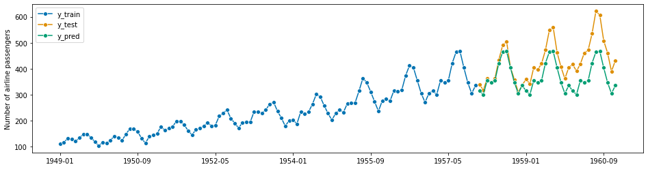
plot_series(y_train, y_test, y_pred, labels=["y_train", "y_test", "y_pred"])
smape_loss(y_pred, y_test)
[8]:
0.23195770387951434
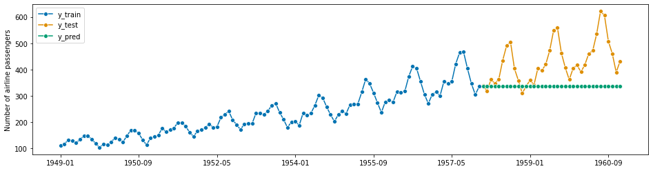
预测同季最后的数值
[9]:
forecaster = NaiveForecaster(strategy="last", sp=12)
forecaster.fit(y_train)
y_pred = forecaster.predict(fh)
plot_series(y_train, y_test, y_pred, labels=["y_train", "y_test", "y_pred"])
smape_loss(y_pred, y_test)
[9]:
0.145427686270316
为什么不直接用scikit-learn?
你可能会有疑问,为什么我们不干脆用scikit-learn来做预测呢?预测说到底不就是一个回归问题吗?
原则上,是的。但是 scikit-learn 并不是为解决预测任务而设计的,所以要小心陷阱!
[10]:
from sklearn.model_selection import train_test_split

y_train, y_test = train_test_split(y)p
plot_series(y_train.sort_index(), y_test.sort_index(), labels=["y_train", "y_test"]);
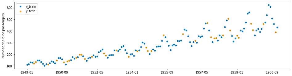
这就导致了
你用来训练机器学习算法的数据恰好有你想要预测的信息。
但是train_test_split(y, shuffle=False)是可以的,这就是sktime中temporal_train_test_split(y)的作用。
[11]:
y_train, y_test = temporal_train_test_split(y)
plot_series(y_train, y_test, labels=["y_train", "y_test"]);
为了使用scikit-learn,我们必须首先将数据转换为所需的表格格式,然后拟合regressor ,最后生成预测。
关键思想:精简
预测通常是通过回归来解决的。这种方法有时被称为还原法,因为我们将预测任务还原为更简单但相关的表格回归任务。这样就可以对预测问题应用任何回归算法。
精简为回归的工作原理如下。我们首先需要将数据转化为所需的表格格式。我们可以通过将训练序列切割成固定长度的窗口,并将它们叠加在一起来实现。我们的目标变量由每个窗口的后续观测值组成。
我们可以写一些代码来做到这一点,例如在M4比赛中。
[12]:
# slightly modified code from the M4 competition
def split_into_train_test(data, in_num, fh):
    """
    Splits the series into train and test sets.

    Each step takes multiple points as inputs
    :param data: an individual TS
    :param fh: number of out of sample points
    :param in_num: number of input points for the forecast
    :return:
    """
    train, test = data[:-fh], data[-(fh + in_num) :]
    x_train, y_train = train[:-1], np.roll(train, -in_num)[:-in_num]
    x_test, y_test = test[:-1], np.roll(test, -in_num)[:-in_num]
    #     x_test, y_test = train[-in_num:], np.roll(test, -in_num)[:-in_num]

    # reshape input to be [samples, time steps, features]
    # (N-NF samples, 1 time step, 1 feature)
    x_train = np.reshape(x_train, (-1, 1))
    x_test = np.reshape(x_test, (-1, 1))
    temp_test = np.roll(x_test, -1)
    temp_train = np.roll(x_train, -1)
    for x in range(1, in_num):
        x_train = np.concatenate((x_train[:-1], temp_train[:-1]), 1)
        x_test = np.concatenate((x_test[:-1], temp_test[:-1]), 1)
        temp_test = np.roll(temp_test, -1)[:-1]
        temp_train = np.roll(temp_train, -1)[:-1]

    return x_train, y_train, x_test, y_test
[13]:
# here we split the time index, rather than the actual values,
# to show how we split the windows
feature_window, target_window, _, _ = split_into_train_test(
    np.arange(len(y)), 10, len(fh)