A Visual Guide to Using BERT for the First Time

https://jalammar.github.io/a-visual-guide-to-using-bert-for-the-first-time/

 

A Visual Guide to Using BERT for the First Time

Translations: Chinese, Korean, Russian

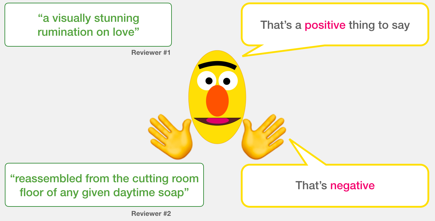
Progress has been rapidly accelerating in machine learning models that process language over the last couple of years. This progress has left the research lab and started powering some of the leading digital products. A great example of this is the recent announcement of how the BERT model is now a major force behind Google Search. Google believes this step (or progress in natural language understanding as applied in search) represents “the biggest leap forward in the past five years, and one of the biggest leaps forward in the history of Search”.

This post is a simple tutorial for how to use a variant of BERT to classify sentences. This is an example that is basic enough as a first intro, yet advanced enough to showcase some of the key concepts involved.

Alongside this post, I’ve prepared a notebook. You can see it here the notebook or run it on colab.

Dataset: SST2

The dataset we will use in this example is SST2, which contains sentences from movie reviews, each labeled as either positive (has the value 1) or negative (has the value 0):

sentence	label
a stirring , funny and finally transporting re imagining of beauty and the beast and 1930s horror films	1
apparently reassembled from the cutting room floor of any given daytime soap	0
they presume their audience won't sit still for a sociology lesson	0
this is a visually stunning rumination on love , memory , history and the war between art and commerce	1
jonathan parker 's bartleby should have been the be all end all of the modern office anomie films	1

Models: Sentence Sentiment Classification

Our goal is to create a model that takes a sentence (just like the ones in our dataset) and produces either 1 (indicating the sentence carries a positive sentiment) or a 0 (indicating the sentence carries a negative sentiment). We can think of it as looking like this:

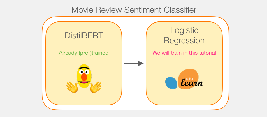
Under the hood, the model is actually made up of two model.

• DistilBERT processes the sentence and passes along some information it extracted from it on to the next model. DistilBERT is a smaller version of BERT developed and open sourced by the team at HuggingFace. It’s a lighter and faster version of BERT that roughly matches its performance.
• The next model, a basic Logistic Regression model from scikit learn will take in the result of DistilBERT’s processing, and classify the sentence as either positive or negative (1 or 0, respectively).

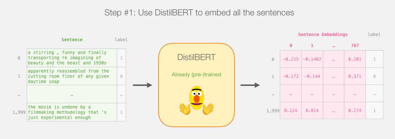
The data we pass between the two models is a vector of size 768. We can think of this of vector as an embedding for the sentence that we can use for classification.

If you’ve read my previous post, Illustrated BERT, this vector is the result of the first position (which receives the [CLS] token as input).

Model Training

While we’ll be using two models, we will only train the logistic regression model. For DistillBERT, we’ll use a model that’s already pre-trained and has a grasp on the English language. This model, however is neither trained not fine-tuned to do sentence classification. We get some sentence classification capability, however, from the general objectives BERT is trained on. This is especially the case with BERT’s output for the first position (associated with the [CLS] token). I believe that’s due to BERT’s second training object – Next sentence classification. That objective seemingly trains the model to encapsulate a sentence-wide sense to the output at the first position. The transformers library provides us with an implementation of DistilBERT as well as pretrained versions of the model.

Tutorial Overview

So here’s the game plan with this tutorial. We will first use the trained distilBERT to generate sentence embeddings for 2,000 sentences.

We will not touch distilBERT after this step. It’s all Scikit Learn from here. We do the usual train/test split on this dataset:

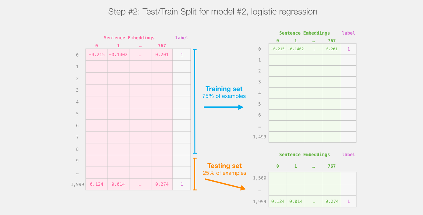
Train/test split for the output of distilBert (model #1) creates the dataset we'll train and evaluate logistic regression on (model #2). Note that in reality, sklearn's train/test split shuffles the examples before making the split, it doesn't just take the first 75% of examples as they appear in the dataset.

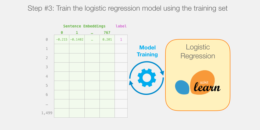
Then we train the logistic regression model on the training set:

How a single prediction is calculated

Before we dig into the code and explain how to train the model, let’s look at how a trained model calculates its prediction.

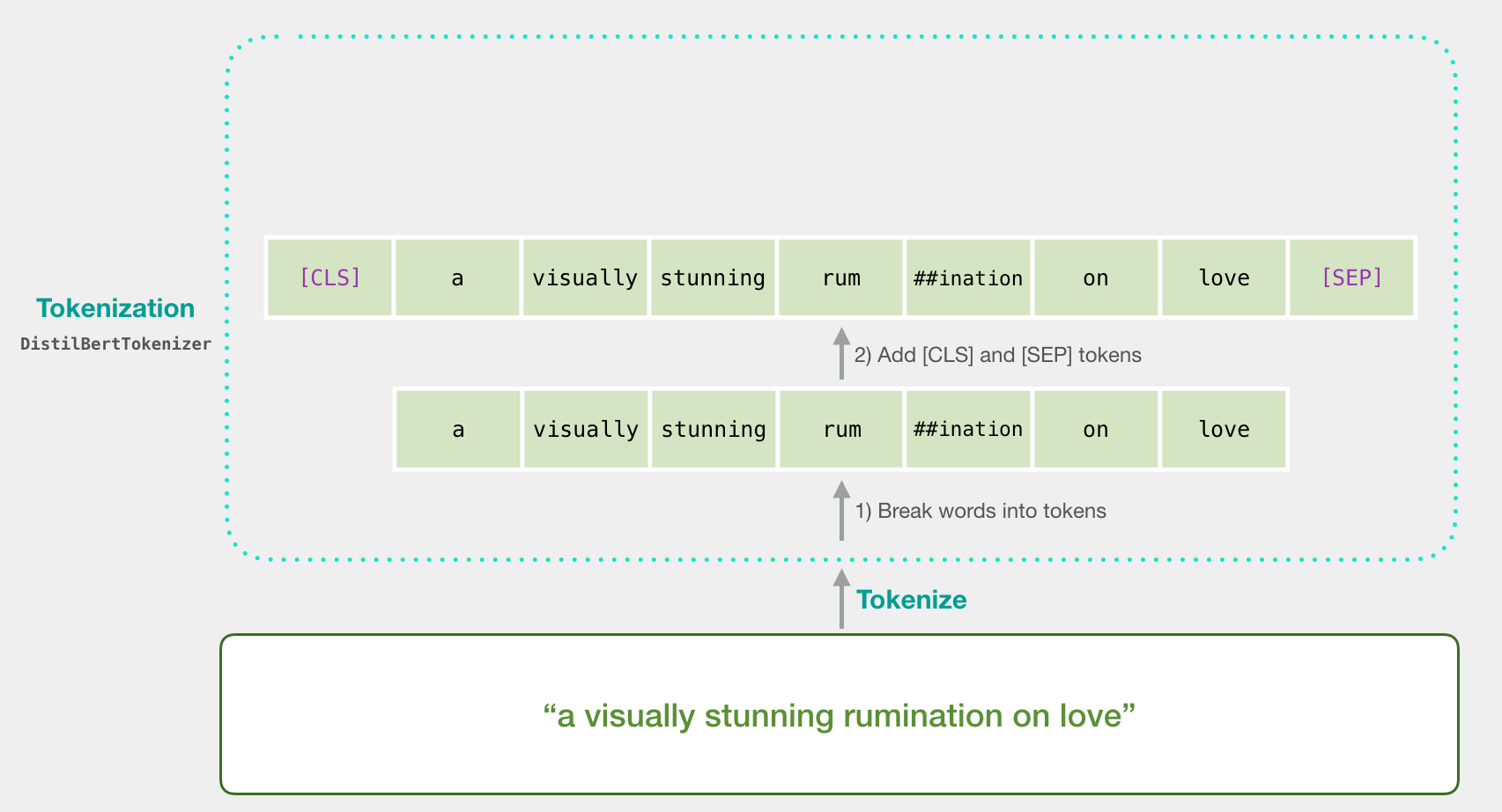
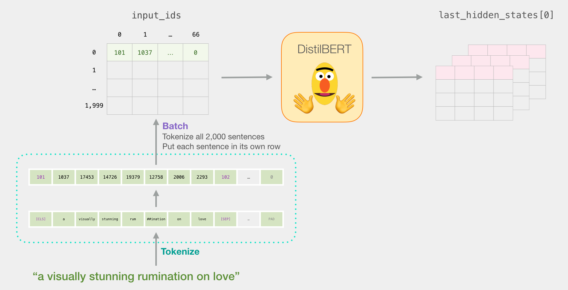
Let’s try to classify the sentence “a visually stunning rumination on love”. The first step is to use the BERT tokenizer to first split the word into tokens. Then, we add the special tokens needed for sentence classifications (these are [CLS] at the first position, and [SEP] at the end of the sentence).

The third step the tokenizer does is to replace each token with its id from the embedding table which is a component we get with the trained model. Read The Illustrated Word2vec for a background on word embeddings.

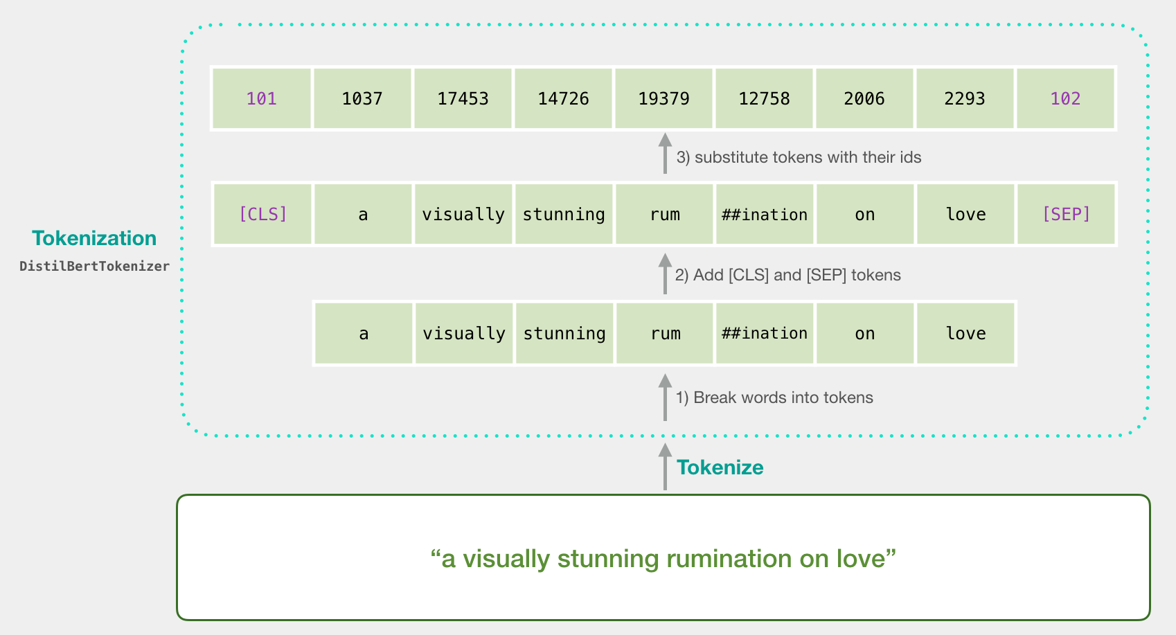
Note that the tokenizer does all these steps in a single line of code:

tokenizer.encode("a visually stunning rumination on love", add_special_tokens=True)

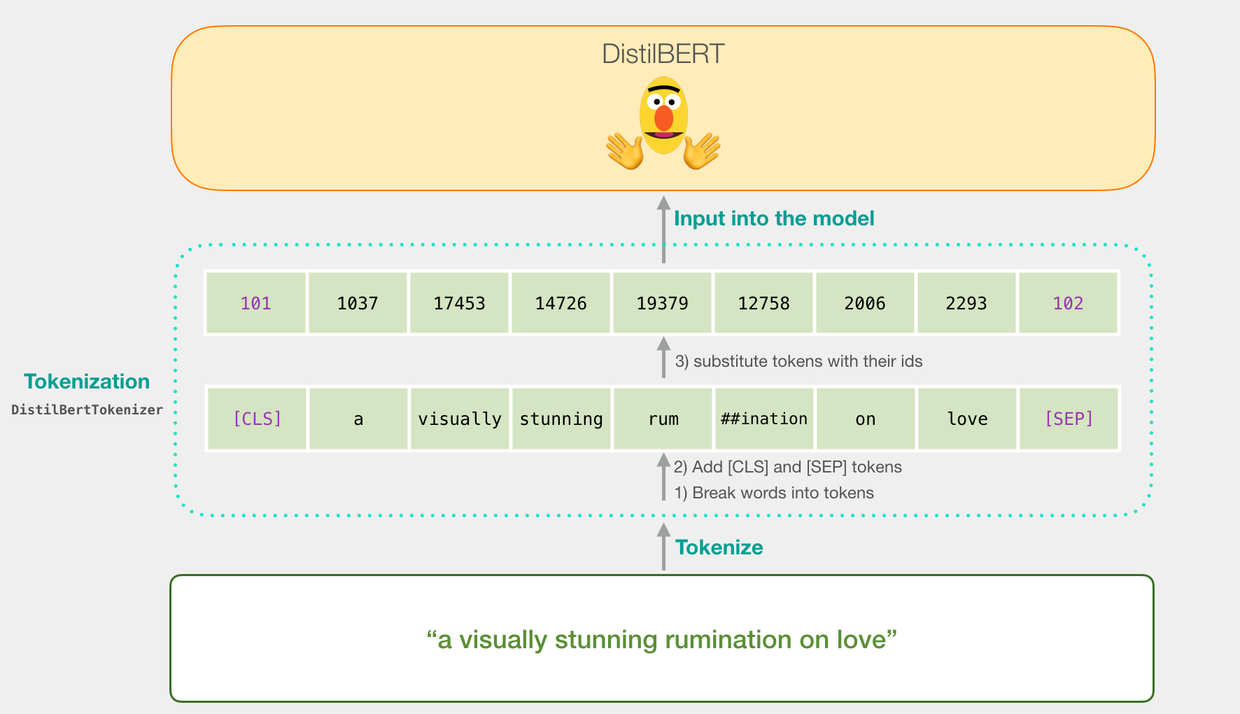
Our input sentence is now the proper shape to be passed to DistilBERT.

If you’ve read Illustrated BERT, this step can also be visualized in this manner:

Flowing Through DistilBERT

Passing the input vector through DistilBERT works just like BERT. The output would be a vector for each input token. each vector is made up of 768 numbers (floats).

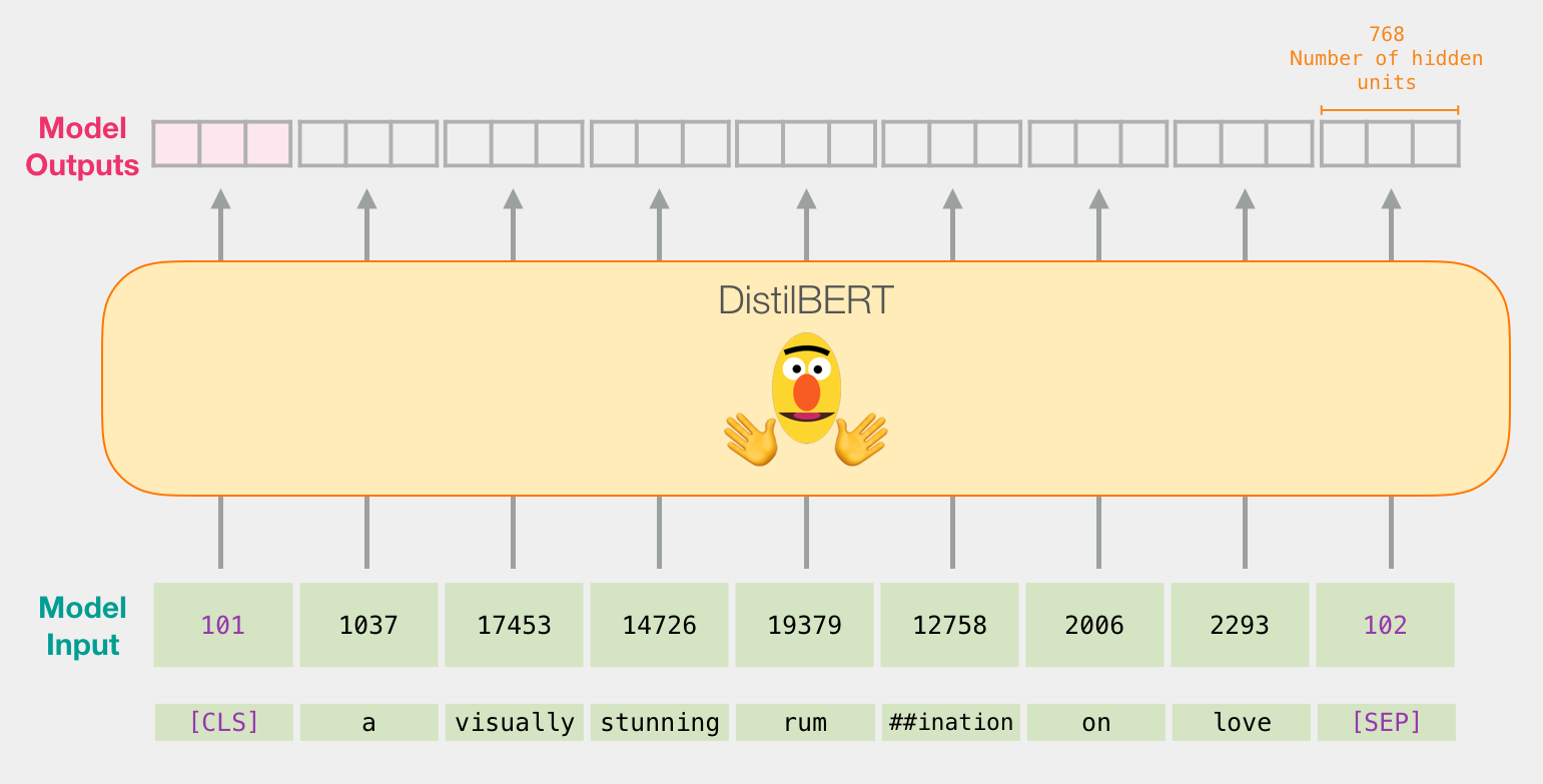
Because this is a sentence classification task, we ignore all except the first vector (the one associated with the [CLS] token). The one vector we pass as the input to the logistic regression model.

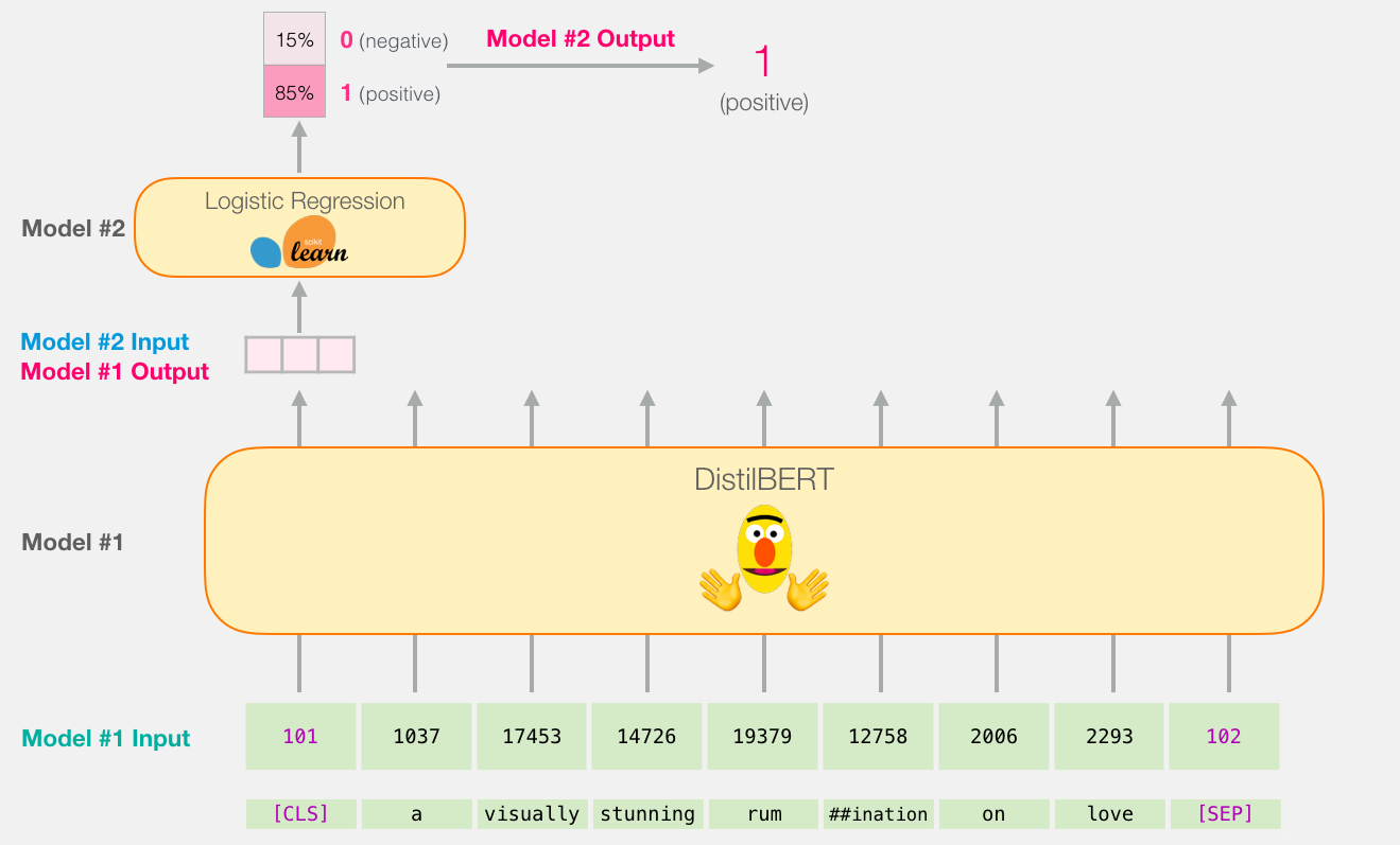
From here, it’s the logistic regression model’s job to classify this vector based on what it learned from its training phase. We can think of a prediction calculation as looking like this:

The training is what we’ll discuss in the next section, along with the code of the entire process.

The Code

In this section we’ll highlight the code to train this sentence classification model. A notebook containing all this code is available on colab and github.

Let’s start by importing the tools of the trade

import numpy as np
import pandas as pd
import torch
import transformers as ppb # pytorch transformers
from sklearn.linear_model import LogisticRegression
from sklearn.model_selection import cross_val_score
from sklearn.model_selection import train_test_split

The dataset is available as a file on github, so we just import it directly into a pandas dataframe

df = pd.read_csv('https://github.com/clairett/pytorch-sentiment-classification/raw/master/data/SST2/train.tsv', delimiter='\t', header=None)

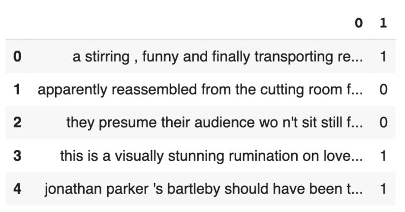
We can use df.head() to look at the first five rows of the dataframe to see how the data looks.

df.head()

Which outputs:

Importing pre-trained DistilBERT model and tokenizer

model_class, tokenizer_class, pretrained_weights = (ppb.DistilBertModel, ppb.DistilBertTokenizer, 'distilbert-base-uncased')

## Want BERT instead of distilBERT? Uncomment the following line:
#model_class, tokenizer_class, pretrained_weights = (ppb.BertModel, ppb.BertTokenizer, 'bert-base-uncased')

# Load pretrained model/tokenizer
tokenizer = tokenizer_class.from_pretrained(pretrained_weights)
model = model_class.from_pretrained(pretrained_weights)

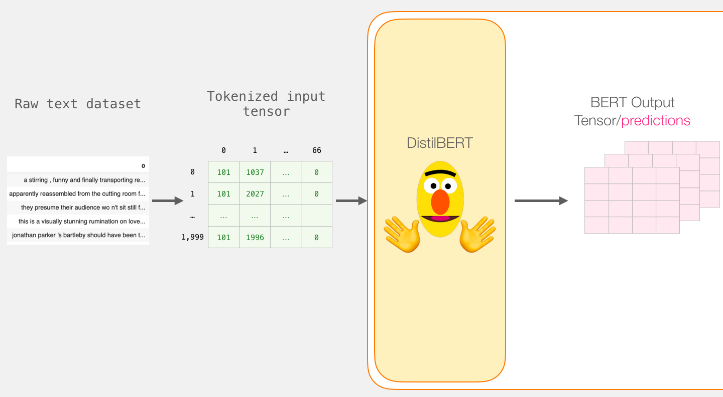
We can now tokenize the dataset. Note that we’re going to do things a little differently here from the example above. The example above tokenized and processed only one sentence. Here, we’ll tokenize and process all sentences together as a batch (the notebook processes a smaller group of examples just for resource considerations, let’s say 2000 examples).

Tokenization

tokenized = df[0].apply((lambda x: tokenizer.encode(x, add_special_tokens=True)))

This turns every sentence into the list of ids.

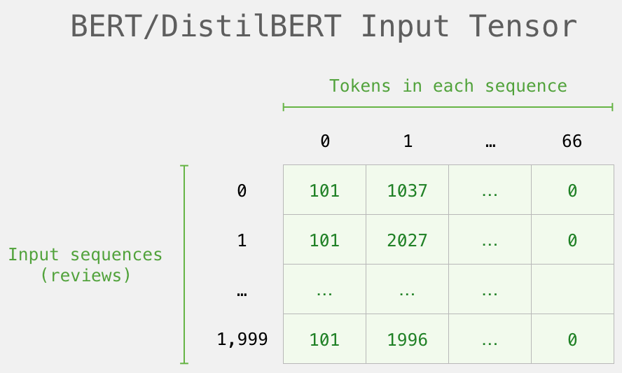
The dataset is currently a list (or pandas Series/DataFrame) of lists. Before DistilBERT can process this as input, we’ll need to make all the vectors the same size by padding shorter sentences with the token id 0. You can refer to the notebook for the padding step, it’s basic python string and array manipulation.

After the padding, we have a matrix/tensor that is ready to be passed to BERT:

Processing with DistilBERT

We now create an input tensor out of the padded token matrix, and send that to DistilBERT

input_ids = torch.tensor(np.array(padded))

with torch.no_grad():
    last_hidden_states = model(input_ids)

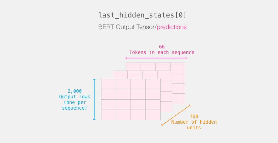
After running this step, last_hidden_states holds the outputs of DistilBERT. It is a tuple with the shape (number of examples, max number of tokens in the sequence, number of hidden units in the DistilBERT model). In our case, this will be 2000 (since we only limited ourselves to 2000 examples), 66 (which is the number of tokens in the longest sequence from the 2000 examples), 768 (the number of hidden units in the DistilBERT model).

Unpacking the BERT output tensor

Let’s unpack this 3-d output tensor. We can first start by examining its dimensions:

Recapping a sentence’s journey

Each row is associated with a sentence from our dataset. To recap the processing path of the first sentence, we can think of it as looking like this:

Slicing the important part

For sentence classification, we’re only only interested in BERT’s output for the [CLS] token, so we select that slice of the cube and discard everything else.

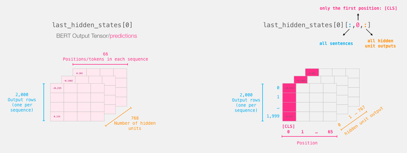
This is how we slice that 3d tensor to get the 2d tensor we’re interested in:

 # Slice the output for the first position for all the sequences, take all hidden unit outputs
features = last_hidden_states[0][:,0,:].numpy()

And now features is a 2d numpy array containing the sentence embeddings of all the sentences in our dataset.

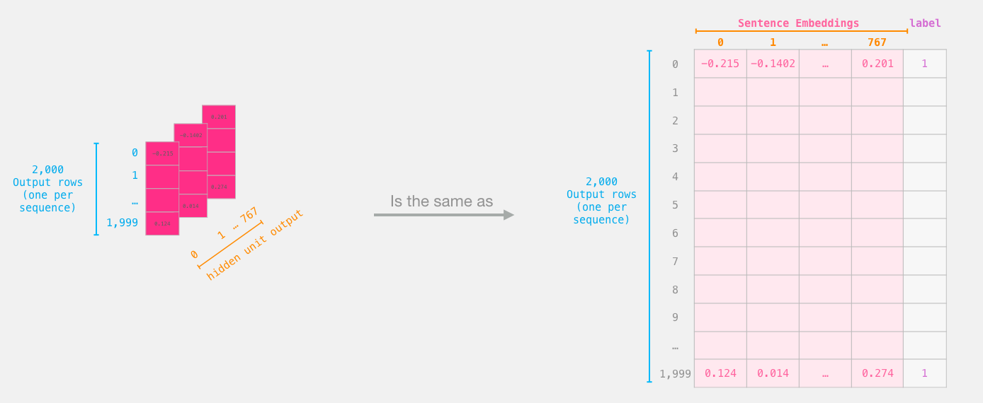
The tensor we sliced from BERT's output

Dataset for Logistic Regression

Now that we have the output of BERT, we have assembled the dataset we need to train our logistic regression model. The 768 columns are the features, and the labels we just get from our initial dataset.

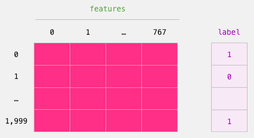
The labeled dataset we use to train the Logistic Regression. The features are the output vectors of BERT for the [CLS] token (position #0) that we sliced in the previous figure. Each row corresponds to a sentence in our dataset, each column corresponds to the output of a hidden unit from the feed-forward neural network at the top transformer block of the Bert/DistilBERT model.

After doing the traditional train/test split of machine learning, we can declare our Logistic Regression model and train it against the dataset.

labels = df[1]
train_features, test_features, train_labels, test_labels = train_test_split(features, labels)

Which splits the dataset into training/testing sets:

Next, we train the Logistic Regression model on the training set.

lr_clf = LogisticRegression()
lr_clf.fit(train_features, train_labels)

Now that the model is trained, we can score it against the test set:

lr_clf.score(test_features, test_labels)

Which shows the model achieves around 81% accuracy.

Score Benchmarks

For reference, the highest accuracy score for this dataset is currently 96.8. DistilBERT can be trained to improve its score on this task – a process called fine-tuning which updates BERT’s weights to make it achieve a better performance in the sentence classification (which we can call the downstream task). The fine-tuned DistilBERT turns out to achieve an accuracy score of 90.7. The full size BERT model achieves 94.9.

The Notebook

Dive right into the notebook or run it on colab.

And that’s it! That’s a good first contact with BERT. The next step would be to head over to the documentation and try your hand at fine-tuning. You can also go back and switch from distilBERT to BERT and see how that works.

Thanks to Clément Delangue, Victor Sanh, and the Huggingface team for providing feedback to earlier versions of this tutorial.

Written on November 26, 2019