
石头减到布
建立一个可以有多个分类的神经网络
第一步:下载数据
wget --no-check-certificate \
    https://storage.googleapis.com/laurencemoroney-blog.appspot.com/rps.zip \
    -O tmp/rps.zip

wget --no-check-certificate \
    https://storage.googleapis.com/laurencemoroney-blog.appspot.com/rps-test-set.zip \
    -O tmp/rps-test-set.zip
第二步:解压并显示数据
import os
import zipfile

# unzip file
local_zip = 'tmp/rps.zip'
zip_ref = zipfile.ZipFile(local_zip, 'r')
zip_ref.extractall('tmp/')
zip_ref.close()

local_zip = 'tmp/rps-test-set.zip'
zip_ref = zipfile.ZipFile(local_zip, 'r')
zip_ref.extractall('tmp/')
zip_ref.close()

rock_dir = os.path.join('tmp/rps/rock')
paper_dir = os.path.join('tmp/rps/paper')
scissors_dir = os.path.join('tmp/rps/scissors')

print('total training rock images:', len(os.listdir(rock_dir)))
print('total training paper images:', len(os.listdir(paper_dir)))
print('total training scissors images:', len(os.listdir(scissors_dir)))

rock_files = os.listdir(rock_dir)
print(rock_files[:10])

paper_files = os.listdir(paper_dir)
print(paper_files[:10])

scissors_files = os.listdir(scissors_dir)
print(scissors_files[:10])
运行结果:
total training rock images: 840
total training paper images: 840
total training scissors images: 840
['rock04-059.png', 'rock01-108.png',
'rock04-065.png', 'rock05ck01-067.png',
'rock05ck01-073.png', 'rock04-071.png',
'rock05ck01-098.png', 'rock02-008.png',
'rock07-k03-013.png', 'rock02-034.png']
['paper03-088.png', 'paper05-026.png', 'paper05-032.png',
'paper03-077.png', 'paper03-063.png', 'paper02-099.png',
'paper04-037.png', 'paper04-023.png', 'paper02-066.png', 'paper02-072.png']
['testscissors03-040.png', 'testscissors03-054.png', 'testscissors03-068.png',
'testscissors03-083.png', 'testscissors03-097.png', 'scissors03-113.png',
'scissors03-107.png', 'testscissors02-051.png', 'testscissors02-045.png', 'scissors01-002.png']
注释: 使用 matplotlib 显示数据
%matplotlib inline

import matplotlib.pyplot as plt
import matplotlib.image as mpimg

pic_index = 2

next_rock = [os.path.join(rock_dir, fname)
                for fname in rock_files[pic_index-2:pic_index]]
next_paper = [os.path.join(paper_dir, fname)
                for fname in paper_files[pic_index-2:pic_index]]
next_scissors = [os.path.join(scissors_dir, fname)
                for fname in scissors_files[pic_index-2:pic_index]]

for i, img_path in enumerate(next_rock+next_paper+next_scissors):
  #print(img_path)
  img = mpimg.imread(img_path)
  plt.imshow(img)
  plt.axis('Off')
  plt.show()
第三步:建立模型
import tensorflow as tf
import keras_preprocessing
from keras_preprocessing import image
from keras_preprocessing.image import ImageDataGenerator

TRAINING_DIR = "tmp/rps/"
training_datagen = ImageDataGenerator(
      rescale = 1./255,
      rotation_range=40,
      width_shift_range=0.2,
      height_shift_range=0.2,
      shear_range=0.2,
      zoom_range=0.2,
      horizontal_flip=True,
      fill_mode='nearest')

VALIDATION_DIR = "tmp/rps-test-set/"
validation_datagen = ImageDataGenerator(rescale = 1./255)

train_generator = training_datagen.flow_from_directory(
    TRAINING_DIR,
    target_size=(150,150),
    class_mode='categorical'
)

validation_generator = validation_datagen.flow_from_directory(
    VALIDATION_DIR,
    target_size=(150,150),
    class_mode='categorical'
)

model = tf.keras.models.Sequential([
    # Note the input shape is the desired size of the image 150x150 with 3 bytes color
    # This is the first convolution
    tf.keras.layers.Conv2D(64, (3,3), activation='relu', input_shape=(150, 150, 3)),
    tf.keras.layers.MaxPooling2D(2, 2),
    # The second convolution
    tf.keras.layers.Conv2D(64, (3,3), activation='relu'),
    tf.keras.layers.MaxPooling2D(2,2),
    # The third convolution
    tf.keras.layers.Conv2D(128, (3,3), activation='relu'),
    tf.keras.layers.MaxPooling2D(2,2),
    # The fourth convolution
    tf.keras.layers.Conv2D(128, (3,3), activation='relu'),
    tf.keras.layers.MaxPooling2D(2,2),
    # Flatten the results to feed into a DNN
    tf.keras.layers.Flatten(),
    tf.keras.layers.Dropout(0.5),
    # 512 neuron hidden layer
    tf.keras.layers.Dense(512, activation='relu'),
    tf.keras.layers.Dense(3, activation='softmax')
])


model.summary()

model.compile(loss = 'categorical_crossentropy', optimizer='rmsprop', metrics=['accuracy'])

history = model.fit_generator(train_generator, epochs=25, validation_data = validation_generator, verbose = 1)

model.save("rps.h5")
运行结果:
Found 2520 images belonging to 3 classes.
Found 372 images belonging to 3 classes.
Model: "sequential_5"
_________________________________________________________________
Layer (type)                 Output Shape              Param #
=================================================================
conv2d_20 (Conv2D)           (None, 148, 148, 64)      1792
_________________________________________________________________
max_pooling2d_20 (MaxPooling (None, 74, 74, 64)        0
_________________________________________________________________
conv2d_21 (Conv2D)           (None, 72, 72, 64)        36928
_________________________________________________________________
max_pooling2d_21 (MaxPooling (None, 36, 36, 64)        0
_________________________________________________________________
conv2d_22 (Conv2D)           (None, 34, 34, 128)       73856
_________________________________________________________________
max_pooling2d_22 (MaxPooling (None, 17, 17, 128)       0
_________________________________________________________________
conv2d_23 (Conv2D)           (None, 15, 15, 128)       147584
_________________________________________________________________
max_pooling2d_23 (MaxPooling (None, 7, 7, 128)         0
_________________________________________________________________
flatten_5 (Flatten)          (None, 6272)              0
_________________________________________________________________
dropout_5 (Dropout)          (None, 6272)              0
_________________________________________________________________
dense_10 (Dense)             (None, 512)               3211776
_________________________________________________________________
dense_11 (Dense)             (None, 3)                 1539
=================================================================
Total params: 3,473,475
Trainable params: 3,473,475
Non-trainable params: 0
_________________________________________________________________
Epoch 1/25
79/79==============================] - 20s 257ms/step - loss: 1.2037 - acc: 0.3786 - val_loss: 1.0084 - val_acc: 0.6344
Epoch 2/25
79/79==============================] - 19s 242ms/step - loss: 0.8781 - acc: 0.6000 - val_loss: 0.3174 - val_acc: 0.9946
Epoch 3/25
79/79==============================] - 20s 250ms/step - loss: 0.5636 - acc: 0.7595 - val_loss: 0.1306 - val_acc: 1.0000
Epoch 4/25
79/79==============================] - 19s 243ms/step - loss: 0.4033 - acc: 0.8397 - val_loss: 0.2548 - val_acc: 0.8414
Epoch 5/25
79/79==============================] - 19s 240ms/step - loss: 0.3114 - acc: 0.8897 - val_loss: 0.0518 - val_acc: 0.9866
Epoch 6/25
79/79==============================] - 20s 251ms/step - loss: 0.2161 - acc: 0.9278 - val_loss: 0.1461 - val_acc: 0.9409
Epoch 7/25
79/79==============================] - 19s 246ms/step - loss: 0.2107 - acc: 0.9282 - val_loss: 0.0579 - val_acc: 0.9892
Epoch 8/25
79/79==============================] - 19s 243ms/step - loss: 0.1796 - acc: 0.9345 - val_loss: 0.0487 - val_acc: 0.9812
Epoch 9/25
79/79==============================] - 20s 252ms/step - loss: 0.1681 - acc: 0.9468 - val_loss: 0.0209 - val_acc: 0.9946
Epoch 10/25
79/79==============================] - 20s 257ms/step - loss: 0.1286 - acc: 0.9532 - val_loss: 0.1703 - val_acc: 0.9328
Epoch 11/25
79/79==============================] - 19s 241ms/step - loss: 0.1457 - acc: 0.9532 - val_loss: 0.0287 - val_acc: 0.9919
Epoch 12/25
79/79==============================] - 19s 241ms/step - loss: 0.1053 - acc: 0.9687 - val_loss: 0.0737 - val_acc: 0.9704
Epoch 13/25
79/79==============================] - 20s 249ms/step - loss: 0.1216 - acc: 0.9603 - val_loss: 0.0290 - val_acc: 0.9866
Epoch 14/25
79/79==============================] - 19s 236ms/step - loss: 0.1651 - acc: 0.9532 - val_loss: 0.0918 - val_acc: 0.9758
Epoch 15/25
79/79==============================] - 19s 236ms/step - loss: 0.0996 - acc: 0.9659 - val_loss: 0.1870 - val_acc: 0.8978
Epoch 16/25
79/79==============================] - 20s 248ms/step - loss: 0.0804 - acc: 0.9702 - val_loss: 0.0228 - val_acc: 0.9839
Epoch 17/25
79/79==============================] - 19s 241ms/step - loss: 0.1079 - acc: 0.9659 - val_loss: 0.0448 - val_acc: 0.9785
Epoch 18/25
79/79==============================] - 19s 240ms/step - loss: 0.1005 - acc: 0.9667 - val_loss: 0.0431 - val_acc: 0.9812
Epoch 19/25
79/79==============================] - 19s 244ms/step - loss: 0.0983 - acc: 0.9698 - val_loss: 0.0627 - val_acc: 0.9785
Epoch 20/25
79/79==============================] - 20s 249ms/step - loss: 0.0830 - acc: 0.9738 - val_loss: 0.3355 - val_acc: 0.8575
Epoch 21/25
79/79==============================] - 19s 245ms/step - loss: 0.1141 - acc: 0.9647 - val_loss: 0.0584 - val_acc: 0.9731
Epoch 22/25
79/79==============================] - 19s 243ms/step - loss: 0.0803 - acc: 0.9750 - val_loss: 0.0380 - val_acc: 0.9812
Epoch 23/25
79/79==============================] - 20s 253ms/step - loss: 0.0762 - acc: 0.9754 - val_loss: 0.3842 - val_acc: 0.9167
Epoch 24/25
79/79==============================] - 19s 246ms/step - loss: 0.0781 - acc: 0.9758 - val_loss: 0.0176 - val_acc: 0.9892
Epoch 25/25
79/79==============================] - 19s 237ms/step - loss: 0.0708 - acc: 0.9810 - val_loss: 0.1145 - val_acc: 0.9543
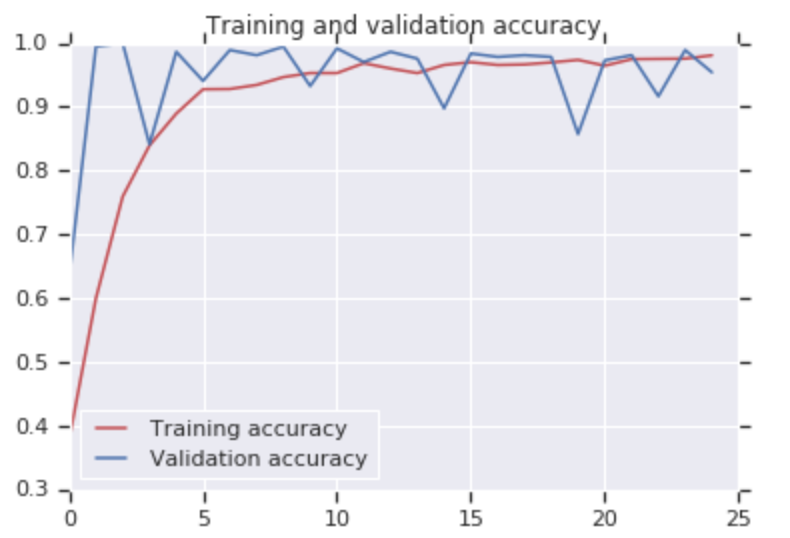
使用图像显示
import matplotlib.pyplot as plt
acc = history.history['acc']
val_acc = history.history['val_acc']
loss = history.history['loss']
val_loss = history.history['val_loss']

epochs = range(len(acc))

plt.plot(epochs, acc, 'r', label='Training accuracy')
plt.plot(epochs, val_acc, 'b', label='Validation accuracy')
plt.title('Training and validation accuracy')
plt.legend(loc=0)
plt.figure()


plt.show()
运行结果
|

 浙公网安备 33010602011771号