卷积神经网络(二)
本例使用神经网络识别人和马的照片
第一步:下载数据
wget --no-check-certificate \
    https://storage.googleapis.com/laurencemoroney-blog.appspot.com/horse-or-human.zip \
    -O /tmp/horse-or-human.zip
运行结果
--2020-01-03 06:15:15-- https://storage.googleapis.com/laurencemoroney-blog.appspot.com/horse-or-human.zip Resolving storage.googleapis.com (storage.googleapis.com)... 108.177.111.128, 2607:f8b0:4001:c15::80 Connecting to storage.googleapis.com (storage.googleapis.com)|108.177.111.128|:443... connected. HTTP request sent, awaiting response... 200 OK Length: 149574867 (143M) [application/zip] Saving to: ‘/tmp/horse-or-human.zip’ /tmp/horse-or-human 100%[===================>] 142.65M 98.5MB/s in 1.4s 2020-01-03 06:15:16 (98.5 MB/s) - ‘/tmp/horse-or-human.zip’ saved [149574867/149574867]
第二步:解压数据
import os
import zipfile

local_zip = '/tmp/horse-or-human.zip'
zip_ref = zipfile.ZipFile(local_zip, 'r')
zip_ref.extractall('/tmp/horse-or-human')
zip_ref.close()
第三步:定义训练集
# Directory with our training horse pictures
train_horse_dir = os.path.join('/tmp/horse-or-human/horses')

# Directory with our training human pictures
train_human_dir = os.path.join('/tmp/horse-or-human/humans')
注释:可以使用 os.listdir 进行查看
train_horse_names = os.listdir(train_horse_dir)
print(train_horse_names[:10])

train_human_names = os.listdir(train_human_dir)
print(train_human_names[:10])
运行结果
['horse38-3.png', 'horse03-0.png', 'horse35-8.png', 'horse04-6.png', 'horse44-6.png', 'horse49-8.png', 'horse14-9.png', 'horse06-5.png', 'horse41-5.png', 'horse04-9.png']
['human14-16.png', 'human15-15.png', 'human11-10.png', 'human10-13.png', 'human07-06.png', 'human17-01.png', 'human09-13.png', 'human09-11.png', 'human05-15.png', 'human04-14.png']
注释: 查看目录中有多少个数目
print('total training horse images:', len(os.listdir(train_horse_dir)))
print('total training human images:', len(os.listdir(train_human_dir)))
运行结果
total training horse images: 500
total training human images: 527
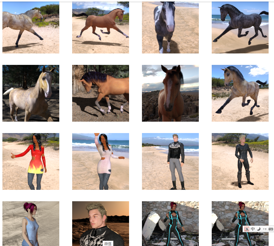
注释: 可以使用 matplotlib 进行照片查看
%matplotlib inline

import matplotlib.pyplot as plt
import matplotlib.image as mpimg

# Parameters for our graph; we'll output images in a 4x4 configuration
nrows = 4
ncols = 4

# Index for iterating over images
pic_index = 0


# Set up matplotlib fig, and size it to fit 4x4 pics
fig = plt.gcf()
fig.set_size_inches(ncols * 4, nrows * 4)

# 8 * 8 列的
pic_index += 8
next_horse_pix = [os.path.join(train_horse_dir, fname)
                for fname in train_horse_names[pic_index-8:pic_index]]
next_human_pix = [os.path.join(train_human_dir, fname)
                for fname in train_human_names[pic_index-8:pic_index]]

for i, img_path in enumerate(next_horse_pix+next_human_pix):
  # Set up subplot; subplot indices start at 1
  sp = plt.subplot(nrows, ncols, i + 1)
  sp.axis('Off') # Don't show axes (or gridlines)

  img = mpimg.imread(img_path)
  plt.imshow(img)

plt.show()
运行结果
第四步:定义模型与网络
import tensorflow as tf

model = tf.keras.models.Sequential([
    # Note the input shape is the desired size of the image 300x300 with 3 bytes color
    # This is the first convolution
    tf.keras.layers.Conv2D(16, (3,3), activation='relu', input_shape=(300, 300, 3)),
    tf.keras.layers.MaxPooling2D(2, 2),
    # The second convolution
    tf.keras.layers.Conv2D(32, (3,3), activation='relu'),
    tf.keras.layers.MaxPooling2D(2,2),
    # The third convolution
    tf.keras.layers.Conv2D(64, (3,3), activation='relu'),
    tf.keras.layers.MaxPooling2D(2,2),
    # The fourth convolution
    tf.keras.layers.Conv2D(64, (3,3), activation='relu'),
    tf.keras.layers.MaxPooling2D(2,2),
    # The fifth convolution
    tf.keras.layers.Conv2D(64, (3,3), activation='relu'),
    tf.keras.layers.MaxPooling2D(2,2),
    # Flatten the results to feed into a DNN
    tf.keras.layers.Flatten(),
    # 512 neuron hidden layer
    tf.keras.layers.Dense(512, activation='relu'),
    # Only 1 output neuron. It will contain a value from 0-1 where 0 for 1 class ('horses') and 1 for the other ('humans')
    tf.keras.layers.Dense(1, activation='sigmoid')
])
注释: 可以使用 model.summary() 方法进行查看
model.summary()
运行结果
Model: "sequential"
_________________________________________________________________
Layer (type)                 Output Shape              Param #
=================================================================
conv2d (Conv2D)              (None, 298, 298, 16)      448
_________________________________________________________________
max_pooling2d (MaxPooling2D) (None, 149, 149, 16)      0
_________________________________________________________________
conv2d_1 (Conv2D)            (None, 147, 147, 32)      4640
_________________________________________________________________
max_pooling2d_1 (MaxPooling2 (None, 73, 73, 32)        0
_________________________________________________________________
conv2d_2 (Conv2D)            (None, 71, 71, 64)        18496
_________________________________________________________________
max_pooling2d_2 (MaxPooling2 (None, 35, 35, 64)        0
_________________________________________________________________
conv2d_3 (Conv2D)            (None, 33, 33, 64)        36928
_________________________________________________________________
max_pooling2d_3 (MaxPooling2 (None, 16, 16, 64)        0
_________________________________________________________________
conv2d_4 (Conv2D)            (None, 14, 14, 64)        36928
_________________________________________________________________
max_pooling2d_4 (MaxPooling2 (None, 7, 7, 64)          0
_________________________________________________________________
flatten (Flatten)            (None, 3136)              0
_________________________________________________________________
dense (Dense)                (None, 512)               1606144
_________________________________________________________________
dense_1 (Dense)              (None, 1)                 513
=================================================================
Total params: 1,704,097
Trainable params: 1,704,097
Non-trainable params: 0
_________________________________________________________________
第五步:编译模型
from tensorflow.keras.optimizers import RMSprop

model.compile(loss='binary_crossentropy',
              optimizer=RMSprop(lr=0.001),
              metrics=['acc'])
第六步: 处理数据
from tensorflow.keras.preprocessing.image import ImageDataGenerator

# All images will be rescaled by 1./255
train_datagen = ImageDataGenerator(rescale=1/255)

# Flow training images in batches of 128 using train_datagen generator
train_generator = train_datagen.flow_from_directory(
        '/tmp/horse-or-human/',  # This is the source directory for training images
        target_size=(300, 300),  # All images will be resized to 150x150
        batch_size=128,
        # Since we use binary_crossentropy loss, we need binary labels
        class_mode='binary')
第七步: 训练模型
history = model.fit_generator(
      train_generator,
      steps_per_epoch=8,
      epochs=15,
      verbose=1)
运行结果
Epoch 1/15
8/8 [==============================] - 8s 1s/step - loss: 1.7235 - acc: 0.5006
Epoch 2/15
8/8 [==============================] - 6s 689ms/step - loss: 0.6713 - acc: 0.6104
Epoch 3/15
8/8 [==============================] - 5s 580ms/step - loss: 0.7703 - acc: 0.6809
Epoch 4/15
8/8 [==============================] - 5s 679ms/step - loss: 0.5567 - acc: 0.6463
Epoch 5/15
8/8 [==============================] - 5s 681ms/step - loss: 1.3130 - acc: 0.7119
Epoch 6/15
8/8 [==============================] - 5s 680ms/step - loss: 0.3521 - acc: 0.8832
Epoch 7/15
8/8 [==============================] - 6s 772ms/step - loss: 0.1969 - acc: 0.9258
Epoch 8/15
8/8 [==============================] - 5s 678ms/step - loss: 0.1722 - acc: 0.9244
Epoch 9/15
8/8 [==============================] - 5s 674ms/step - loss: 0.1337 - acc: 0.9444
Epoch 10/15
8/8 [==============================] - 5s 678ms/step - loss: 0.5653 - acc: 0.8409
Epoch 11/15
8/8 [==============================] - 6s 779ms/step - loss: 0.4015 - acc: 0.8350
Epoch 12/15
8/8 [==============================] - 6s 688ms/step - loss: 0.1242 - acc: 0.9633
Epoch 13/15
8/8 [==============================] - 5s 597ms/step - loss: 0.0500 - acc: 0.9742
Epoch 14/15
8/8 [==============================] - 6s 689ms/step - loss: 0.0549 - acc: 0.9800
Epoch 15/15
8/8 [==============================] - 6s 798ms/step - loss: 0.3984 - acc: 0.8818
运行模型, 从本地文件中上传照片
import numpy as np
from google.colab import files
from keras.preprocessing import image

uploaded = files.upload()

for fn in uploaded.keys():

  # predicting images
  path = '/content/' + fn
  img = image.load_img(path, target_size=(300, 300))
  x = image.img_to_array(img)
  x = np.expand_dims(x, axis=0)

  images = np.vstack([x])
  classes = model.predict(images, batch_size=10)
  print(classes[0])
  if classes[0]>0.5:
    print(fn + " is a human")
  else:
    print(fn + " is a horse")
查看运行过程
import numpy as np
import random
from tensorflow.keras.preprocessing.image import img_to_array, load_img

# Let's define a new Model that will take an image as input, and will output
# intermediate representations for all layers in the previous model after
# the first.
successive_outputs = [layer.output for layer in model.layers[1:]]
#visualization_model = Model(img_input, successive_outputs)
visualization_model = tf.keras.models.Model(inputs = model.input, outputs = successive_outputs)
# Let's prepare a random input image from the training set.
horse_img_files = [os.path.join(train_horse_dir, f) for f in train_horse_names]
human_img_files = [os.path.join(train_human_dir, f) for f in train_human_names]
img_path = random.choice(horse_img_files + human_img_files)

img = load_img(img_path, target_size=(300, 300))  # this is a PIL image
x = img_to_array(img)  # Numpy array with shape (150, 150, 3)
x = x.reshape((1,) + x.shape)  # Numpy array with shape (1, 150, 150, 3)

# Rescale by 1/255
x /= 255

# Let's run our image through our network, thus obtaining all
# intermediate representations for this image.
successive_feature_maps = visualization_model.predict(x)

# These are the names of the layers, so can have them as part of our plot
layer_names = [layer.name for layer in model.layers]

# Now let's display our representations
for layer_name, feature_map in zip(layer_names, successive_feature_maps):
  if len(feature_map.shape) == 4:
    # Just do this for the conv / maxpool layers, not the fully-connected layers
    n_features = feature_map.shape[-1]  # number of features in feature map
    # The feature map has shape (1, size, size, n_features)
    size = feature_map.shape[1]
    # We will tile our images in this matrix
    display_grid = np.zeros((size, size * n_features))
    for i in range(n_features):
      # Postprocess the feature to make it visually palatable
      x = feature_map[0, :, :, i]
      x -= x.mean()
      x /= x.std()
      x *= 64
      x += 128
      x = np.clip(x, 0, 255).astype('uint8')
      # We'll tile each filter into this big horizontal grid
      display_grid[:, i * size : (i + 1) * size] = x
    # Display the grid
    scale = 20. / n_features
    plt.figure(figsize=(scale * n_features, scale))
    plt.title(layer_name)
    plt.grid(False)
    plt.imshow(display_grid, aspect='auto', cmap='viridis')
第八步:清除数据
import os, signal
os.kill(os.getpid(), signal.SIGKILL)

 浙公网安备 33010602011771号