卷积神经网络

1.卷积神经网络概念

卷积网络是一种非常智能的网络结构，并且具有不变性。

有两个重要概念

* 卷积(Convolutions)

* 最大池化(MaxPooling)

1.1 卷积的概念

卷积是指向图像应用滤波器的过程。

假设有一张灰度图像，假设其有6 * 6 橡素，每个像素值在 [0,255] 之间。

图1-1 一张灰度图像转换成6 * 6 的矩阵

圈积网络的原理是创建另一个数字网络，叫做核或滤波器。

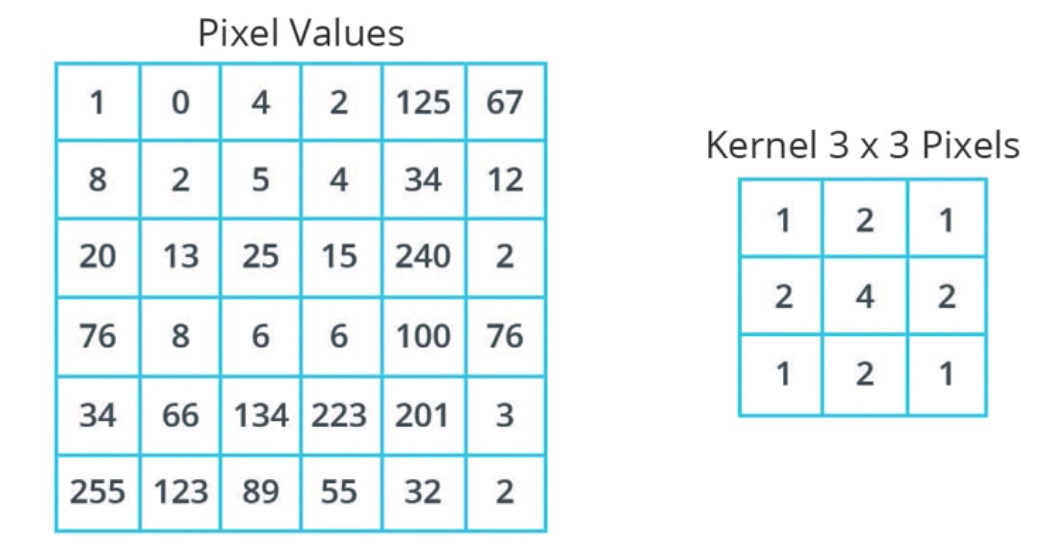
图1-2 创建另一个3 * 3 数字矩阵

然后用该核矩阵扫描 6 * 6 的矩阵，扫描过程如下

假设我们要扫描第3行第3列的值25，执行卷积运算

第一步：将该值周边的区域与kernel 一一对应

图1-3 选中与 kernel 相同大小区域

第二步：对25执行卷积运算

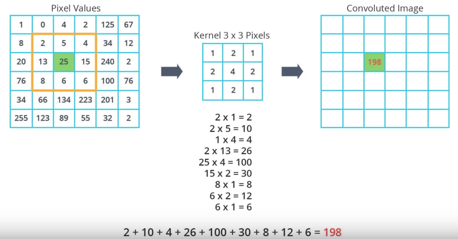
图1-4 执行卷积运算

如果对于边缘的像素，通常有两种做法

第一种，直接忽略，但会损失图像

第二种，在边缘填充0

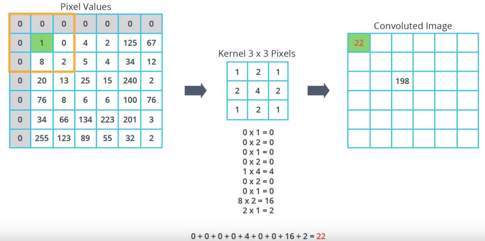
图1-5 卷积网络填充过程

最终计算结果如下

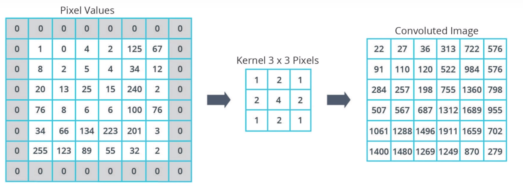
图1-6 卷积网络计算最终结果

资源资料

https://towardsdatascience.com/a-comprehensive-guide-to-convolutional-neural-networks-the-eli5-way-3bd2b1164a53

1.2 最大池化(MaxPooling)

简言之，通过总结区域，减小输入图像大小的流程。

为了使用MaxPooling ，必须先要定义好两个参数

池大小与步长，然后选择该区域中最大的值。

池大小，本例选择的是2 * 2 的矩阵

步长指的是在图像上滑动窗口的间隔像素数量。

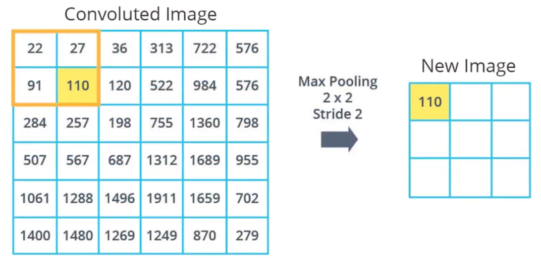
图1-7 将卷积运算后的图片使用池化减小

最终的结果是，我们将得到一个比之前更小的图像

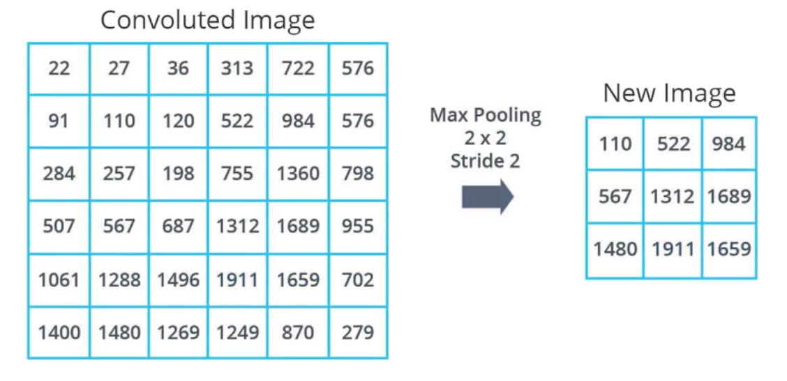
图1-8 经过最大池化后的结果

最终图像大小取决于你所使用的池大小与步长。

2. Coding

使用卷积神经网络(Convolutional Neural Networks， CNN)来进行照片分类。

第一步：安装并导入数据包

from __future__ import absolute_import, division, print_function, unicode_literals

import tensorflow as tf

# Import TensorFlow Datasets
import tensorflow_datasets as tfds
tfds.disable_progress_bar()

# Helper libraries
import math
import numpy as np
import matplotlib.pyplot as plt


import logging
logger = tf.get_logger()
logger.setLevel(logging.ERROR)

第二步：设置输入、输出，训练，测试数据

dataset, metadata = tfds.load('fashion_mnist', as_supervised=True, with_info=True)
train_dataset, test_dataset = dataset['train'], dataset['test']


class_names = ['T-shirt/top', 'Trouser', 'Pullover', 'Dress', 'Coat',
               'Sandal',      'Shirt',   'Sneaker',  'Bag',   'Ankle boot']


num_train_examples = metadata.splits['train'].num_examples
num_test_examples = metadata.splits['test'].num_examples
print("Number of training examples: {}".format(num_train_examples))
print("Number of test examples:     {}".format(num_test_examples))

运行结果

Number of training examples: 60000
Number of test examples: 10000

第三步：序列化数据

def normalize(images, labels):
  images = tf.cast(images, tf.float32)
  images /= 255
  return images, labels

# The map function applies the normalize function to each element in the train
# and test datasets
train_dataset =  train_dataset.map(normalize)
test_dataset  =  test_dataset.map(normalize)

# The first time you use the dataset, the images will be loaded from disk
# Caching will keep them in memory, making training faster
train_dataset =  train_dataset.cache()
test_dataset  =  test_dataset.cache()

第四步：选中一张图片，查看是否正确

# Take a single image, and remove the color dimension by reshaping
for image, label in test_dataset.take(1):
  break
image = image.numpy().reshape((28,28))

# Plot the image - voila a piece of fashion clothing
plt.figure()
plt.imshow(image, cmap=plt.cm.binary)
plt.colorbar()
plt.grid(False)
plt.show()

输出结果：

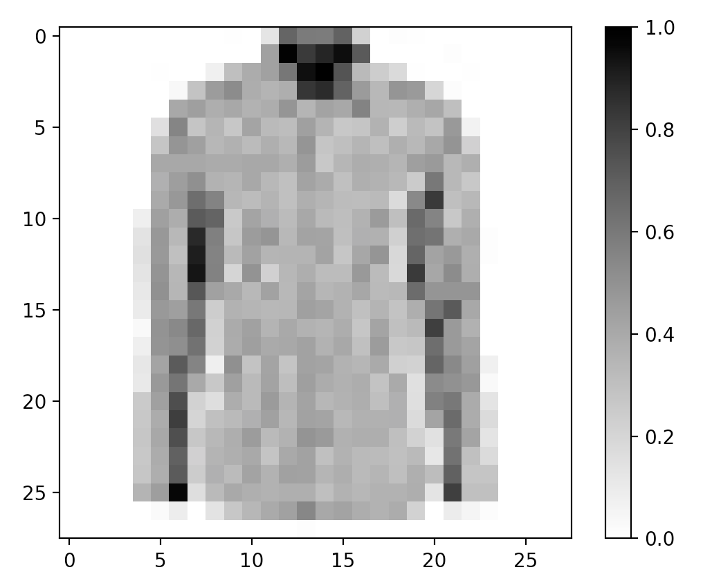
图2-1 查看Fashion-Minist 图片

第五步：输出25张照片，查看照片是否正确

plt.figure(figsize=(10,10))
i = 0
for (image, label) in test_dataset.take(25):
    image = image.numpy().reshape((28,28))
    plt.subplot(5,5,i+1)
    plt.xticks([])
    plt.yticks([])
    plt.grid(False)
    plt.imshow(image, cmap=plt.cm.binary)
    plt.xlabel(class_names[label])
    i += 1
plt.show()

输出结果

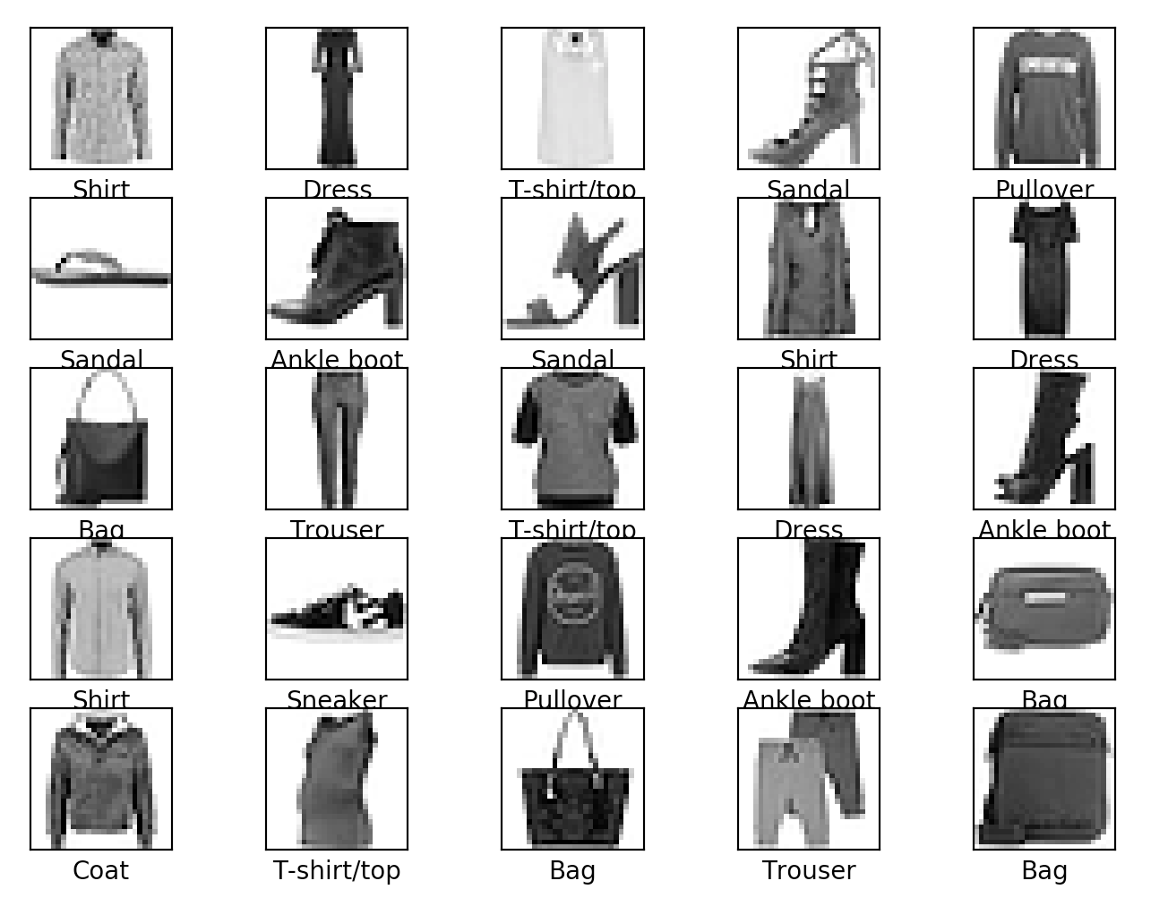
图2-2 查看25 张照片输出结果

第六步：设置模型CNN层

model = tf.keras.Sequential([
    tf.keras.layers.Conv2D(32, (3,3), padding='same', activation=tf.nn.relu,
                           input_shape=(28, 28, 1)),
    tf.keras.layers.MaxPooling2D((2, 2), strides=2),
    tf.keras.layers.Conv2D(64, (3,3), padding='same', activation=tf.nn.relu),
    tf.keras.layers.MaxPooling2D((2, 2), strides=2),
    tf.keras.layers.Flatten(),
    tf.keras.layers.Dense(128, activation=tf.nn.relu),
    tf.keras.layers.Dense(10,  activation=tf.nn.softmax)
])

* "卷积（convolutions）" tf.keras.layers.Conv2D 和 MaxPooling2D— Network start with two pairs of Conv/MaxPool.

第一层，使用Conv2D过滤器，大小是 3*3 的矩阵，边界使用0填充，并且输出32张卷积图像

第二层，使用最大池化，池大小为 2 * 2，步长为2。

第三层，同样使用 3 * 3 的矩阵，使用32张图像做为输入创建64张卷积图像。

* 输出 tf.keras.layers.Dense — 128个单元神经, 10个输出类另，输出 osftmax即概率模型. 输出值为 [0,1], 总和是1

第七步：编译模型

model.compile(optimizer='adam',
              loss='sparse_categorical_crossentropy',
              metrics=['accuracy'])

第八步：训练模型

BATCH_SIZE = 32
train_dataset = train_dataset.repeat().shuffle(num_train_examples).batch(BATCH_SIZE)
test_dataset = test_dataset.batch(BATCH_SIZE)

model.fit(train_dataset, epochs=10, steps_per_epoch=math.ceil(num_train_examples/BATCH_SIZE))

执行结果：

Train for 1875 steps
Epoch 1/10
1875/1875 [==============================] - 82s 44ms/step - loss: 0.3701 - accuracy: 0.8648
Epoch 2/10
1875/1875 [==============================] - 80s 43ms/step - loss: 0.2421 - accuracy: 0.9114
Epoch 3/10
1875/1875 [==============================] - 78s 41ms/step - loss: 0.1941 - accuracy: 0.9292
Epoch 4/10
1875/1875 [==============================] - 69s 37ms/step - loss: 0.1566 - accuracy: 0.9423
Epoch 5/10
1875/1875 [==============================] - 71s 38ms/step - loss: 0.1311 - accuracy: 0.9514
Epoch 6/10
1875/1875 [==============================] - 70s 38ms/step - loss: 0.1033 - accuracy: 0.9613
Epoch 7/10
1875/1875 [==============================] - 70s 38ms/step - loss: 0.0832 - accuracy: 0.9690
Epoch 8/10
1875/1875 [==============================] - 71s 38ms/step - loss: 0.0664 - accuracy: 0.9757
Epoch 9/10
1875/1875 [==============================] - 73s 39ms/step - loss: 0.0508 - accuracy: 0.9815
Epoch 10/10
1875/1875 [==============================] - 73s 39ms/step - loss: 0.0455 - accuracy: 0.9836

第九步：使用测试集进行测试

test_loss, test_accuracy = model.evaluate(test_dataset, steps=math.ceil(num_test_examples/32))
print('Accuracy on test dataset:', test_accuracy)

运行结果

313/313 [==============================] - 5s 16ms/step - loss: 0.3474 - accuracy: 0.9234
Accuracy on test dataset: 0.9234

posted @ 2020-01-01 18:05 elewei 阅读(461) 评论(0) 编辑收藏举报

会员力量，点亮园子希望

刷新页面返回顶部

David

卷积神经网络

1.卷积神经网络概念

1.1 卷积的概念

1.2 最大池化(MaxPooling)

2. Coding