03 - Fashion MINIST识别衣服(多分类问题)

目标：使用Fashion MINIST 数据集训练一个可以自动识别衣服的神经网络。

Fashion MINIST 数据集参考链接

https://github.com/zalandoresearch/fashion-mnist

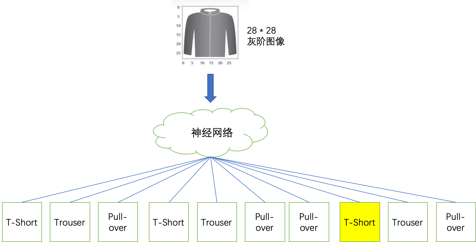
图 1-1 创建一个可以识别衣服的神经网络

分析步骤

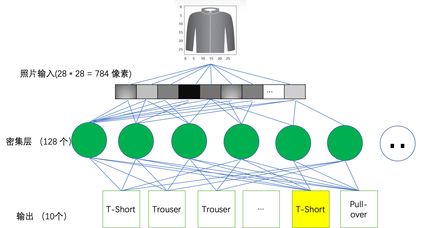
图1-2 分析结果

测试集一共有70000条，使用60000条进行训练， 10000条进行测试。

第一步：数据表示，这个过程叫做扁平化(Flatten)

将输入的图像转换成一个由784个橡素组成的一维数组

使用代码表示如下

tf.keras.layers.Flatten(input_shape=(28,28,1))

第二步：密集层，我们有128个单元

tf.keras.layers.Dense(128, activtion=tf.nn.relu)

第三步：输出表示

标签	类别	概率（总和 = 1）
0	T-Shirt
1	Trouser
2	Pullover
3	Dress
4	Coat
5	Sandal
6	Shirt
7	Sneaker
8	Bag
9	Ankle Boot

即神经网络最终的输出结果是一个概率分布，测试数据中每个照片对应的类别的概率分布

tf.keras.layers.Dense(10, activation=tf.nn.softmax)

Coading

第一步：安装环境

pip install tenserflow
pip install -U tensorflow_datasets

第二步：导入数据包

# Import TensorFlow Datasets
import tensorflow_datasets as tfds
tfds.disable_progress_bar()

# Helper libraries
import math
import numpy as np
import matplotlib.pyplot as plt

第三步：导入Fashion Minist数据集

# Import Fashion minist dataset
dataset, metadata = tfds.load('fashion_mnist', as_supervised=True, with_info=True)
train_dataset, test_dataset = dataset['train'], dataset['test']

打印查看minst 信息

print(metadata)

tfds.core.DatasetInfo(
    name='fashion_mnist',
    version=1.0.0,
    description='Fashion-MNIST is a dataset of Zalando's article images consisting of a training set of 60,000 examples and a test set of 10,000 examples. Each example is a 28x28 grayscale image, associated with a label from 10 classes.',
    homepage='https://github.com/zalandoresearch/fashion-mnist',
    features=FeaturesDict({
        'image': Image(shape=(28, 28, 1), dtype=tf.uint8),
        'label': ClassLabel(shape=(), dtype=tf.int64, num_classes=10),
    }),
    total_num_examples=70000,
    splits={
        'test': 10000,
        'train': 60000,
    },
    supervised_keys=('image', 'label'),
    citation="""@article{DBLP:journals/corr/abs-1708-07747,
      author    = {Han Xiao and
                   Kashif Rasul and
                   Roland Vollgraf},
      title     = {Fashion-MNIST: a Novel Image Dataset for Benchmarking Machine Learning
                   Algorithms},
      journal   = {CoRR},
      volume    = {abs/1708.07747},
      year      = {2017},
      url       = {http://arxiv.org/abs/1708.07747},
      archivePrefix = {arXiv},
      eprint    = {1708.07747},
      timestamp = {Mon, 13 Aug 2018 16:47:27 +0200},
      biburl    = {https://dblp.org/rec/bib/journals/corr/abs-1708-07747},
      bibsource = {dblp computer science bibliography, https://dblp.org}
    }""",
    redistribution_info=,
)

print(dataset)

{
 'test': <_OptionsDataset shapes: ((28, 28, 1), ()), types: (tf.uint8, tf.int64)>, 
 'train': <_OptionsDataset shapes: ((28, 28, 1), ()), types: (tf.uint8, tf.int64)>
}

查看单张照片信息

[[  0   0   0   0   0   0   0   0   0   1   0  32 172 151 150 176  56   0
    2   1   0   0   0   0   0   0   0   0]
 [  0   0   0   0   0   0   0   0   0   0   0 111 252 211 227 243 183   0
    0   0   0   2   0   0   0   0   0   0]
 [  0   0   0   0   0   1   0   0  19  78  99 111 155 242 255 188  83  61
   46   1   0   0   1   0   0   0   0   0]
 [  0   0   0   0   0   0   9  73 117 133  98  90  97 213 222 175 118  85
  123 119  50   4   0   0   0   0   0   0]
 [  0   0   0   0   0   0 103 113  97 103  91  98 124  89 109 104 143  87
   85  96 105  78   0   0   0   0   0   0]
 [  0   0   0   0   0  39 140  71  89  68 108  83  80 112  90  67  70  91
   59  83  73 120  16   0   0   0   0   0]
 [  0   0   0   0   0  71 124 112  87  93  82  96  85 124  70  78  89  78
   96  86 103 125  57   0   0   0   0   0]
 [  0   0   0   0   0 103 103 103 100 100 104 104  96 117  67  88  98  96
   89 113 119  86  96   0   0   0   0   0]
 [  0   0   0   0   0  94 115 129  92  89 103  86  75 109 100  75  96  92
   85  64 154  86  67   0   0   0   0   0]
 [  0   0   0   0   0 101 121 164 143  87  81  90  76  96  89  81  80  83
   45 137 211  77  86   0   0   0   0   0]
 [  0   0   0   0  20 112  98 181 173  66 108  94  82 104  83  79  92 118
   77 168 141  67  96   0   0   0   0   0]
 [  0   0   0   0  35 121  86 224 146  69 117 124  86 109 107  78  94  93
   58 163 158  96 102   2   0   0   0   0]
 [  0   0   0   0  38 120  76 232 143  83 110  89  90  90 109  69 105 123
   48 172 109 120  96   3   0   0   0   0]
 [  0   0   0   0  33 125  87 237 144  52 126  57  87  97  81  81 120  82
   47 211 105 134  97   0   0   0   0   0]
 [  0   0   0   0  29 128  88 186 111 102  85 110  86 108  88  92 105  83
   85 165 124 124 124   0   0   0   0   0]
 [  0   0   0   0  25 120 113 154  61  92  89  86  87 112 107  92  76  90
   73  97 156 183 103   0   0   0   0   0]
 [  0   0   0   0   7 126 137 170  56 100 111  90 102  91  89  98  69 108
   76  83 206 119  93   0   0   0   0   0]
 [  0   0   0   0  20 125 131 160  55  99 114 101 104 110  92 104  75 117
   67  69 164 119 108   0   0   0   0   0]
 [  0   0   0   0  30 107 181 141  20 129  73 108  72 110 107  92  88 101
   58  55 172 137 112  19   0   0   0   0]
 [  0   0   0   0  27 120 156 102  67 112  83 109  79 113  99  93  98  73
  101  38 135 128 121   8   0   0   0   0]
 [  0   0   0   0  65 112 194  55  41  98  83 118  90 109  87  92  97  77
   94  40 145 154 100  34   0   0   0   0]
 [  0   0   0   0  67  99 208  52  76  83  94 111  87 110 108  86  93  93
   94  43 108 167  99  43   0   0   0   0]
 [  0   0   0   0  69 103 193  68  85  97 117  83  91 125 119  93  97  97
   78  55  37 153 107  34   0   0   0   0]
 [  0   0   0   0  67  99 177  57  90  96 102  72 102 110  76  92  83  82
   75  83  30 160  75  45   0   0   0   0]
 [  0   0   0   0  69  97 181  62  94  82 109  92 111 110  89  97  83  89
   78  96  80 177  70  70   0   0   0   0]
 [  0   0   0   0  90 115 246  41  83 102  96  91  96  96  78  92  87  91
   91  97  34 206  76  75   0   0   0   0]
 [  0   0   0   0   0   6  23   0  35  68  87 101 111 139 104 109  98  91
   99  55   0  24  13   4   0   0   0   0]
 [  0   0   0   0   0   0   0   0   0   0   0   0   0   2   0   0   0   0
    0   0   0   0   0   0   0   0   0   0]]

所有的值都在[0,255]之间

第四步：设置输出数据

class_names = ['T-shirt/top', 'Trouser', 'Pullover', 'Dress', 'Coat',
               'Sandal',      'Shirt',   'Sneaker',  'Bag',   'Ankle boot']

第五步：查看数据

num_train_examples = metadata.splits['train'].num_examples
num_test_examples = metadata.splits['test'].num_examples
print("Number of training examples: {}".format(num_train_examples))
print("Number of test examples:     {}".format(num_test_examples))

运行结果

Number of training examples: 60000
Number of test examples: 10000

有 60000条训练数据， 10000 条测试数据

第六步：处理数据

每个数据的像素值在[0, 255]之间，为了能让模型损失值最小，将值参数化到[0,1]

所以这里创建normalize函数，且应用到每张照片

def normalize(images, labels):
  images = tf.cast(images, tf.float32)
  images /= 255
  return images, labels

# The map function applies the normalize function to each element in the train
# and test datasets
train_dataset =  train_dataset.map(normalize)
test_dataset  =  test_dataset.map(normalize)

# The first time you use the dataset, the images will be loaded from disk
# Caching will keep them in memory, making training faster
train_dataset =  train_dataset.cache()
test_dataset  =  test_dataset.cache()

第七步：查看一张照片

# Take a single image, and remove the color dimension by reshaping
for image, label in test_dataset.take(1):
  break
image = image.numpy().reshape((28,28))

# Plot the image - voila a piece of fashion clothing
plt.figure()
plt.imshow(image, cmap=plt.cm.binary)
plt.colorbar()
plt.grid(False)
plt.show()

运行结果

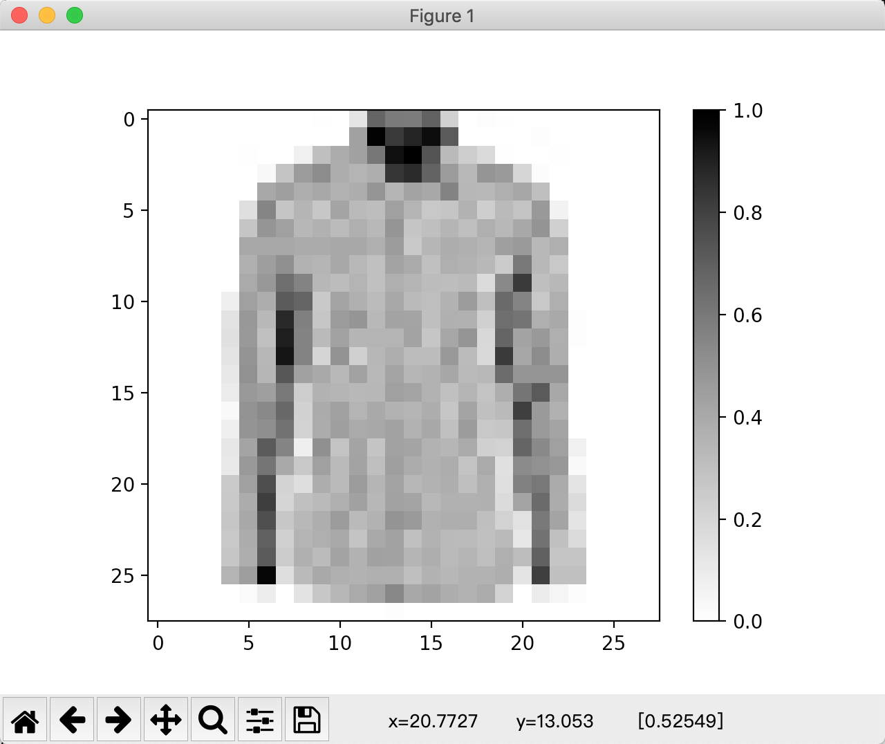
图1-3单张照片显示结果

第八步：显示前25张照片，确认数据是否正确

plt.figure(figsize=(10,10))
i = 0
for (image, label) in test_dataset.take(25):
    image = image.numpy().reshape((28,28))
    plt.subplot(5,5,i+1)
    plt.xticks([])
    plt.yticks([])
    plt.grid(False)
    plt.imshow(image, cmap=plt.cm.binary)
    plt.xlabel(class_names[label])
    i += 1
plt.show()

运行结果

图1-4 确认后的照片

第九步：设置训练模型

model = tf.keras.Sequential([
    tf.keras.layers.Flatten(input_shape=(28, 28, 1)),
    tf.keras.layers.Dense(128, activation=tf.nn.relu),
    tf.keras.layers.Dense(10,  activation=tf.nn.softmax)
])

这个网络拥有3层

第一层 input ，即输入层 - tf.keras.layers.Flatten

这层将28 * 28 的二维矩阵变换成一维的 728 像素的一维数组。

第二层，隐藏的层， tf.keras.layers.Dense , 密集连接 128 个单元的神经，每个单元节点都会从第一层中接收

输入信息，使用权重信息来学习，并计算出结果。

第三层，输出层，tf.keras.layers.Dense ，一个10个节点的输出概率层(softmax)，每个节点表示一个服饰类别。

每个节点根据输入信息与权重值，学习并计算出[0，1]之间的一个值，所有节点的值相加为1。

如果在第二层增加更多的神经单元，则准确率会更高，比如实验加到1024个，时间会更长，但精度会提高。

第十步：编译模型

model.compile(optimizer='adam',
              loss='sparse_categorical_crossentropy',
              metrics=['accuracy'])

在编译模型之前，需要定义损失函数与优化函数。

第十一步：训练模型

BATCH_SIZE = 32
train_dataset = train_dataset.repeat().shuffle(num_train_examples).batch(BATCH_SIZE)
test_dataset = test_dataset.batch(BATCH_SIZE)

model.fit(train_dataset, epochs=5, steps_per_epoch=math.ceil(num_train_examples/BATCH_SIZE))

* 使用接口 train_dataset.repeat() 函数循环执行

* dataset.shuffle(60000) 可以让模型数据乱序，让模型无法从读取顺序进行学习。

* dataset.batch(32) 告诉模型使用32个照片来更新一次

* 训练模型使用 model.fit 函数， epochs = 5 限制模型最多循环学习5次，所以最多可以有 5 * 60000 = 300000 样本

输出结果

Train for 1875 steps
Epoch 1/5
1875/1875 [==============================] - 15s 8ms/step - loss: 0.5014 - accuracy: 0.8243
Epoch 2/5
1875/1875 [==============================] - 5s 2ms/step - loss: 0.3696 - accuracy: 0.8680
Epoch 3/5
1875/1875 [==============================] - 5s 3ms/step - loss: 0.3353 - accuracy: 0.8775
Epoch 4/5
1875/1875 [==============================] - 5s 2ms/step - loss: 0.3124 - accuracy: 0.8862
Epoch 5/5
1875/1875 [==============================] - 5s 2ms/step - loss: 0.2969 - accuracy: 0.8913

如果修改测试epochs的值，将该值增加到30 ，会有什么效果

Train for 1875 steps
Epoch 1/30
1875/1875 [==============================] - 14s 7ms/step - loss: 0.4932 - accuracy: 0.8260
Epoch 2/30
1875/1875 [==============================] - 4s 2ms/step - loss: 0.3762 - accuracy: 0.8633
Epoch 3/30
1875/1875 [==============================] - 4s 2ms/step - loss: 0.3342 - accuracy: 0.8785
Epoch 4/30
1875/1875 [==============================] - 4s 2ms/step - loss: 0.3165 - accuracy: 0.8834
Epoch 5/30
1875/1875 [==============================] - 4s 2ms/step - loss: 0.2951 - accuracy: 0.8915
Epoch 6/30
1875/1875 [==============================] - 4s 2ms/step - loss: 0.2796 - accuracy: 0.8960
Epoch 7/30
1875/1875 [==============================] - 4s 2ms/step - loss: 0.2640 - accuracy: 0.9021
Epoch 8/30
1875/1875 [==============================] - 4s 2ms/step - loss: 0.2585 - accuracy: 0.9040
Epoch 9/30
1875/1875 [==============================] - 5s 2ms/step - loss: 0.2468 - accuracy: 0.9081
Epoch 10/30
1875/1875 [==============================] - 4s 2ms/step - loss: 0.2354 - accuracy: 0.9133
Epoch 11/30
1875/1875 [==============================] - 5s 2ms/step - loss: 0.2326 - accuracy: 0.9133
Epoch 12/30
1875/1875 [==============================] - 4s 2ms/step - loss: 0.2267 - accuracy: 0.9155
Epoch 13/30
1875/1875 [==============================] - 4s 2ms/step - loss: 0.2124 - accuracy: 0.9195
Epoch 14/30
1875/1875 [==============================] - 4s 2ms/step - loss: 0.2117 - accuracy: 0.9212
Epoch 15/30
1875/1875 [==============================] - 5s 2ms/step - loss: 0.2039 - accuracy: 0.9233
Epoch 16/30
1875/1875 [==============================] - 4s 2ms/step - loss: 0.1980 - accuracy: 0.9256
Epoch 17/30
1875/1875 [==============================] - 4s 2ms/step - loss: 0.1953 - accuracy: 0.9282
Epoch 18/30
1875/1875 [==============================] - 4s 2ms/step - loss: 0.1868 - accuracy: 0.9311
Epoch 19/30
1875/1875 [==============================] - 4s 2ms/step - loss: 0.1857 - accuracy: 0.9307
Epoch 20/30
1875/1875 [==============================] - 4s 2ms/step - loss: 0.1773 - accuracy: 0.9330
Epoch 21/30
1875/1875 [==============================] - 4s 2ms/step - loss: 0.1727 - accuracy: 0.9359
Epoch 22/30
1875/1875 [==============================] - 5s 2ms/step - loss: 0.1690 - accuracy: 0.9359
Epoch 23/30
1875/1875 [==============================] - 4s 2ms/step - loss: 0.1666 - accuracy: 0.9379
Epoch 24/30
1875/1875 [==============================] - 4s 2ms/step - loss: 0.1651 - accuracy: 0.9390
Epoch 25/30
1875/1875 [==============================] - 4s 2ms/step - loss: 0.1604 - accuracy: 0.9398
Epoch 26/30
1875/1875 [==============================] - 4s 2ms/step - loss: 0.1528 - accuracy: 0.9428
Epoch 27/30
1875/1875 [==============================] - 4s 2ms/step - loss: 0.1554 - accuracy: 0.9419
Epoch 28/30
1875/1875 [==============================] - 4s 2ms/step - loss: 0.1466 - accuracy: 0.9444
Epoch 29/30
1875/1875 [==============================] - 4s 2ms/step - loss: 0.1433 - accuracy: 0.9464
Epoch 30/30
1875/1875 [==============================] - 4s 2ms/step - loss: 0.1449 - accuracy: 0.9449

精度值有值会增，有时会减。这种现象叫做过拟合。

将第二层神经单元增加到1024个

Train for 1875 steps
Epoch 1/30
1875/1875 [==============================] - 20s 11ms/step - loss: 0.4686 - accuracy: 0.8305
Epoch 2/30
1875/1875 [==============================] - 13s 7ms/step - loss: 0.3521 - accuracy: 0.8698
Epoch 3/30
1875/1875 [==============================] - 11s 6ms/step - loss: 0.3201 - accuracy: 0.8834
Epoch 4/30
1875/1875 [==============================] - 11s 6ms/step - loss: 0.3010 - accuracy: 0.8888
Epoch 5/30
1875/1875 [==============================] - 11s 6ms/step - loss: 0.2772 - accuracy: 0.8969
Epoch 6/30
1875/1875 [==============================] - 11s 6ms/step - loss: 0.2618 - accuracy: 0.9017
Epoch 7/30
1875/1875 [==============================] - 11s 6ms/step - loss: 0.2556 - accuracy: 0.9040
Epoch 8/30
1875/1875 [==============================] - 11s 6ms/step - loss: 0.2388 - accuracy: 0.9102
Epoch 9/30
1875/1875 [==============================] - 11s 6ms/step - loss: 0.2304 - accuracy: 0.9146
Epoch 10/30
1875/1875 [==============================] - 11s 6ms/step - loss: 0.2210 - accuracy: 0.9161
Epoch 11/30
1875/1875 [==============================] - 11s 6ms/step - loss: 0.2124 - accuracy: 0.9202
Epoch 12/30
1875/1875 [==============================] - 11s 6ms/step - loss: 0.2076 - accuracy: 0.9230
Epoch 13/30
1875/1875 [==============================] - 11s 6ms/step - loss: 0.1937 - accuracy: 0.9269
Epoch 14/30
1875/1875 [==============================] - 11s 6ms/step - loss: 0.1882 - accuracy: 0.9291
Epoch 15/30
1875/1875 [==============================] - 11s 6ms/step - loss: 0.1836 - accuracy: 0.9309
Epoch 16/30
1875/1875 [==============================] - 11s 6ms/step - loss: 0.1742 - accuracy: 0.9345
Epoch 17/30
1875/1875 [==============================] - 11s 6ms/step - loss: 0.1712 - accuracy: 0.9358
Epoch 18/30
1875/1875 [==============================] - 11s 6ms/step - loss: 0.1674 - accuracy: 0.9372
Epoch 19/30
1875/1875 [==============================] - 11s 6ms/step - loss: 0.1648 - accuracy: 0.9377
Epoch 20/30
1875/1875 [==============================] - 11s 6ms/step - loss: 0.1523 - accuracy: 0.9424
Epoch 21/30
1875/1875 [==============================] - 11s 6ms/step - loss: 0.1520 - accuracy: 0.9437
Epoch 22/30
1875/1875 [==============================] - 11s 6ms/step - loss: 0.1475 - accuracy: 0.9449
Epoch 23/30
1875/1875 [==============================] - 11s 6ms/step - loss: 0.1435 - accuracy: 0.9464
Epoch 24/30
1875/1875 [==============================] - 11s 6ms/step - loss: 0.1376 - accuracy: 0.9481
Epoch 25/30
1875/1875 [==============================] - 11s 6ms/step - loss: 0.1363 - accuracy: 0.9489
Epoch 26/30
1875/1875 [==============================] - 11s 6ms/step - loss: 0.1315 - accuracy: 0.9514
Epoch 27/30
1875/1875 [==============================] - 11s 6ms/step - loss: 0.1298 - accuracy: 0.9510
Epoch 28/30
1875/1875 [==============================] - 11s 6ms/step - loss: 0.1225 - accuracy: 0.9538
Epoch 29/30
1875/1875 [==============================] - 11s 6ms/step - loss: 0.1219 - accuracy: 0.9543
Epoch 30/30
1875/1875 [==============================] - 11s 6ms/step - loss: 0.1170 - accuracy: 0.9549

如果当精度达到95%时，我就想停下来，该如何停下来？使用可以callback函数

import tensorflow as tf
print(tf.__version__)

class myCallback(tf.keras.callbacks.Callback):
  def on_epoch_end(self, epoch, logs={}):
    if(logs.get('loss')<0.4):
      print("\nReached 95% accuracy so cancelling training!")
      self.model.stop_training = True

callbacks = myCallback()
mnist = tf.keras.datasets.fashion_mnist
(training_images, training_labels), (test_images, test_labels) = mnist.load_data()
training_images=training_images/255.0
test_images=test_images/255.0
model = tf.keras.models.Sequential([
  tf.keras.layers.Flatten(),
  tf.keras.layers.Dense(512, activation=tf.nn.relu),
  tf.keras.layers.Dense(10, activation=tf.nn.softmax)
])
model.compile(optimizer='adam', loss='sparse_categorical_crossentropy')
model.fit(training_images, training_labels, epochs=5, callbacks=[callbacks])

运行结果

Train for 1875 steps
Epoch 1/30
1875/1875 [==============================] - 23s 12ms/step - loss: 0.4622 - accuracy: 0.8345
Epoch 2/30
1875/1875 [==============================] - 15s 8ms/step - loss: 0.3535 - accuracy: 0.8707
Epoch 3/30
1875/1875 [==============================] - 13s 7ms/step - loss: 0.3215 - accuracy: 0.8822
Epoch 4/30
1875/1875 [==============================] - 12s 6ms/step - loss: 0.2937 - accuracy: 0.8914
Epoch 5/30
1875/1875 [==============================] - 12s 6ms/step - loss: 0.2731 - accuracy: 0.8980
Epoch 6/30
1875/1875 [==============================] - 12s 6ms/step - loss: 0.2631 - accuracy: 0.9031
Epoch 7/30
1875/1875 [==============================] - 12s 6ms/step - loss: 0.2494 - accuracy: 0.9059
Epoch 8/30
1875/1875 [==============================] - 12s 6ms/step - loss: 0.2414 - accuracy: 0.9089
Epoch 9/30
1875/1875 [==============================] - 12s 6ms/step - loss: 0.2249 - accuracy: 0.9161
Epoch 10/30
1875/1875 [==============================] - 12s 6ms/step - loss: 0.2183 - accuracy: 0.9177
Epoch 11/30
1875/1875 [==============================] - 12s 6ms/step - loss: 0.2102 - accuracy: 0.9211
Epoch 12/30
1875/1875 [==============================] - 12s 6ms/step - loss: 0.2024 - accuracy: 0.9229
Epoch 13/30
1875/1875 [==============================] - 14s 7ms/step - loss: 0.1935 - accuracy: 0.9272
Epoch 14/30
1875/1875 [==============================] - 10s 5ms/step - loss: 0.1827 - accuracy: 0.9303
Epoch 15/30
1875/1875 [==============================] - 10s 5ms/step - loss: 0.1820 - accuracy: 0.9309
Epoch 16/30
1875/1875 [==============================] - 12s 6ms/step - loss: 0.1779 - accuracy: 0.9327
Epoch 17/30
1875/1875 [==============================] - 12s 6ms/step - loss: 0.1704 - accuracy: 0.9362
Epoch 18/30
1875/1875 [==============================] - 12s 6ms/step - loss: 0.1637 - accuracy: 0.9383
Epoch 19/30
1875/1875 [==============================] - 11s 6ms/step - loss: 0.1584 - accuracy: 0.9392
Epoch 20/30
1875/1875 [==============================] - 11s 6ms/step - loss: 0.1545 - accuracy: 0.9419
Epoch 21/30
1875/1875 [==============================] - 11s 6ms/step - loss: 0.1538 - accuracy: 0.9428
Epoch 22/30
1870/1875 [============================>.] - ETA: 0s - loss: 0.1446 - accuracy: 0.9454 
Reached 95% accuracy so cancelling training!
1875/1875 [==============================] - 11s 6ms/step - loss: 0.1447 - accuracy: 0.9453

第十二步：使用测试样本进行测试，查看模型的可靠性

test_loss, test_accuracy = model.evaluate(test_dataset, steps=math.ceil(num_test_examples/32))
print('Accuracy on test dataset:', test_accuracy)

输出结果

313/313 [==============================] - 2s 7ms/step - loss: 0.3525 - accuracy: 0.8745
Accuracy on test dataset: 0.8745

此值要比训练值低，但是是正常的。

第十三步：使用模型预测

for test_images, test_labels in test_dataset.take(1):
  test_images = test_images.numpy()
  test_labels = test_labels.numpy()
  predictions = model.predict(test_images)

print(predictions.shape)
print(predictions[0])
print(np.argmax(predictions[0]))

输出结果

(32, 10)

[1.8186693e-05 3.9807421e-07 5.6698783e-03 9.7840610e-05 6.5031536e-02
5.2955219e-08 9.2917830e-01 4.5559503e-09 3.7619016e-06 1.8750285e-10]

上衣的可能性最大

6 -> shirt

posted @ 2019-12-31 00:05 elewei 阅读(1770) 评论(0) 编辑收藏举报

会员力量，点亮园子希望

刷新页面返回顶部

David

03 - Fashion MINIST识别衣服(多分类问题)