tensorflow2.0——常用的函数（包括tf.Variable）

一、常用函数

1、转换tensor数据类型

import tensorflow as tf

a=tf.constant(1.0)
b=tf.cast(a,dtype='int32')
print(a)
print(b)

输出:

tf.Tensor(1.0, shape=(), dtype=float32)
tf.Tensor(1, shape=(), dtype=int32)

2、tensor元素的最大值、最小值、求和与均值

import tensorflow as tf

a=tf.constant([[1,1],[2,2]])

a_min=tf.reduce_min(a)    # 张量元素的最小值
a_max=tf.reduce_max(a)    # 张量元素的最大值
a_mean=tf.reduce_mean(a)   # 张量元素的均值
a_sum=tf.reduce_sum(a)    # 张量元素的和

a_row_sum=tf.reduce_sum(a,axis=0)    # 张量列（第1维度）元素的和
a_col_sum=tf.reduce_sum(a,axis=1)    # 张量行（第2维度）元素的和

print('张量a:\n',a)
print('行求和：\n',a_row_sum)
print('列求和：\n',a_col_sum)

输出：

张量a:
 tf.Tensor(
[[1 1]
 [2 2]], shape=(2, 2), dtype=int32)
行求和：
 tf.Tensor([3 3], shape=(2,), dtype=int32)
列求和：
 tf.Tensor([2 4], shape=(2,), dtype=int32)

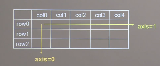
　　参数说明：axis可以定义操作的方向。在矩阵中axis=0表示跨行，对各个列进行求和操作。通常axis=0对应的是tensor.shape的第一个维度。示例图如下：

3、变量的定义与创建

　　TensorFlow中，如果要对一个参数进行训练，那么这个参数必须是一个变量类tf.Variable，tf.Variable类会在反向传播的时候进行梯度计算并保存梯度信息。

import tensorflow as tf

bias = tf.Variable(initial_value=tf.constant(1.0))  # 定义一个逻辑回归的偏倚

4、tensor的数学运算

import tensorflow as tf
a = tf.constant([[1.0, 2.0], [3.0, 4.0]])
b = tf.ones([2, 2])

a_add_b = tf.add(a, b)  # 张量对应元素相加
# a_add_b = a + b  # 张量对应元素相加
a_subtract_b = tf.subtract(a, b)  # 张量对应元素相减
# a_subtract_b = a-b  # 张量对应元素相减
a_multiply_b = tf.multiply(a, b)  # 张量对应元素相乘
# a_subtract_b = a*b  # 张量对应元素相减
a_divide_b = tf.divide(a, b)  # 张量对应元素相除
# a_divide_b = a/b  # 张量对应元素相除
a_square = tf.square(a)  # 张量元素平方
a_pow = tf.pow(a, y=3)  # 张量元素求3次方
# a_pow = a**3  # 张量元素求3次方
a_sqrt = tf.sqrt(a)  # 张量元素开方
a_sqrt = tf.sqrt(a)  # 张量元素开方
a_matmul_b = tf.matmul(a, b)  # 矩阵乘法

print('a:\n',a)
print('b:\n',b)
print('对应元素乘:\n',a_multiply_b)
print('矩阵乘法:\n',a_matmul_b)

输出结果：

a:
 tf.Tensor(
[[1. 2.]
 [3. 4.]], shape=(2, 2), dtype=float32)
b:
 tf.Tensor(
[[1. 1.]
 [1. 1.]], shape=(2, 2), dtype=float32)
对应元素乘:
 tf.Tensor(
[[1. 2.]
 [3. 4.]], shape=(2, 2), dtype=float32)
矩阵乘法:
 tf.Tensor(
[[3. 3.]
 [7. 7.]], shape=(2, 2), dtype=float32)

tips：只有当张量shape相同时才能做四则运算。

5、数据集的加载与处理

import tensorflow as tf
import numpy as np

# 构建数据集
x = np.array(np.arange(1, 7)).reshape(3, 2)
y = np.array(list('ABC')).reshape([3, 1])
data = np.concatenate([x, y], axis=1)
print('生成的数据集为:\n', data)

dataset = tf.data.Dataset.from_tensor_slices((x, y))  # 对数据（x，y）进行切片，将每一个变量特征与标签组成一组

# 切片中的每个元素都是一组（特征,标签）对
print('切片的每一组的内容:')
for element in dataset:
    print(element)


# 定义一个对x、y进行操作的函数，用于dataset.map函数
def process(x, y):
    '''
    :param x: dataset中的x
    :param y: dataset中的y
    :return: 返回值是x,y元祖
    '''
    print('process传入的x：', x)
    print('process传入的y:', y)
    return x, y


dataset.shuffle(3)  # 打乱数据
dataset.map(process)  # 数据进行操作preprocess
dataset.batch(3)  # 定义数据集每批次大小

输出结果为:

生成的数据集为:
 [['1' '2' 'A']
 ['3' '4' 'B']
 ['5' '6' 'C']]

切片的每一组的内容:
(<tf.Tensor: shape=(2,), dtype=int32, numpy=array([1, 2])>, <tf.Tensor: shape=(1,), dtype=string, numpy=array([b'A'], dtype=object)>)
(<tf.Tensor: shape=(2,), dtype=int32, numpy=array([3, 4])>, <tf.Tensor: shape=(1,), dtype=string, numpy=array([b'B'], dtype=object)>)
(<tf.Tensor: shape=(2,), dtype=int32, numpy=array([5, 6])>, <tf.Tensor: shape=(1,), dtype=string, numpy=array([b'C'], dtype=object)>)

process传入的x： Tensor("args_0:0", shape=(2,), dtype=int32)
process传入的y: Tensor("args_1:0", shape=(1,), dtype=string)

总结：

tf.data.Dataset.from_tensor_slices((x, y))，用来对数据进行切片，形成x-y的特征标签对。

```
Dataset.shuffle()，用来打乱数据
```

dataset.map(func)，用来处理dataset加载的数据，map里面的函数func必须要有参数个数必须要和dataset的组成个数相同（这里组成是x、y所以参数为2），因为map传入func的参数个数等于组成个数。

dataset.batch(3)，用来确定每个批次的大小，训练神经网络时，数据经常是分批次训练的。

6、梯度（导数）的计算

import tensorflow as tf

x1 = tf.constant(1.0)
x2 = tf.Variable(1.0)

# 只使用一次tape计算梯度，计算y1在x1=1.0的一阶导数
with tf.GradientTape(persistent=False) as tape:
    tape.watch(x1)  # 对非tf.Variable类的数据需要加入监控才能够训练
    y1 = x1 ** 2    # y需要在梯度带上下文管理器上才可以被计算，如果不在梯度带内无法被监控，计算结果为None
dy1_dx1 = tape.gradient(target=y1, sources=x1)

print('dy1_dx1一阶导数:', dy1_dx1)

# 使用多次tape计算梯度，计算两个一阶导数
with tf.GradientTape(persistent=True) as tape2:
    tape2.watch(x1)  # 对非tf.Variable类的数据需要加入监控才能够训练
    y1 = x1 ** 2
    y2 = x2 ** 3
dy1_dx1 = tape2.gradient(target=y1, sources=x1)
dy2_dx2 = tape2.gradient(target=y2, sources=x2)

print('dy1_dx1一阶导数:', dy1_dx1)
print('dy2_dx2一阶导数:', dy2_dx2)

# 二阶导数
with tf.GradientTape() as tape4:
    tape4.watch(x1)  # 由于是二阶导数，二阶梯度带需要先监控x1，不然二阶求导tape4得不到一阶求导tape3的结果，输出为None
    with tf.GradientTape() as tape3:
        tape3.watch(x1)  # 对非tf.Variable类的数据需要加入监控才能够训练
        y1 = x1 ** 2
    dy1_dx1_1 = tape3.gradient(y1, x1)
dy1_dx1_2 = tape4.gradient(dy1_dx1_1, x1)

print('dy3_dx1_2的二阶导数为:',dy1_dx1_2)

输出结果：

dy1_dx1一阶导数: tf.Tensor(2.0, shape=(), dtype=float32)
dy1_dx1一阶导数: tf.Tensor(2.0, shape=(), dtype=float32)
dy2_dx2一阶导数: tf.Tensor(3.0, shape=(), dtype=float32)
dy3_dx1_2的二阶导数为: tf.Tensor(2.0, shape=(), dtype=float32)

注意事项：

with tf.GradientTape() as tape构建的是一个梯度带上下文处理器，其中tf.GradientTape(persistent，watch_accessed_variables)的参数persistent表示是否可多次计算梯度，参数watch_accessed_variables表示自动监控tf.Variable类可训练的变量。

对于非tf.Variable类张量计算梯度时，需要进行监控，如上述代码在梯度带上下文处理器中添加tape.watch( x1)。
对于y变量，只有y变量的声明在上下文管理器中才能进行梯度计算，否则无法计算。

7、One-hot编码（独热编码）

import tensorflow as tf

y=tf.constant([1,2,3,1])    # y有三个类别
y_trans=tf.one_hot(y,depth=3)   # 定义独热编码的深度为3，即用3个位数表示类别
print(y_trans)

输出结果：

tf.Tensor(
[[0. 1. 0.]
 [0. 0. 1.]
 [0. 0. 0.]
 [0. 1. 0.]], shape=(4, 3), dtype=float32)

函数：

　　tf.one_hot(indices, depth, on_value=None, off_value=None, axis=None, dtype=None, name=None)

参数说明：

indices：表示输入的多个数值，通常是矩阵形式。

depth：编码的深度，即独热编码的位数。

on_value：当y归属为这一类时，独热编码在这个位置的表示值，默认为1。

off_value：当y不属于这一类时，独热编码在这个位置的表示值，默认为0。

8、最大元素、最小元素的索引

　　当我们对y进行One-hot编码后，我们一般是认为最大值1所在的位置即为y的类别。同理，神经网络输出层用sofmax函数作为激活函数后，也取预测值y最大值的位置对应的类别作为预测的分类。这时候我们就需要知道最大值是对应的哪一个位置。

import tensorflow as tf

a=tf.constant([1,1,2,3,1])   
a_trans=tf.one_hot(a,3) # 转换为独热编码
a_pre=tf.argmax(a_trans,axis=1) # 最大值所在的位置

print(a)
print(a_trans)
print(a_pre)

输出结果:

tf.Tensor([1 1 2 3 1], shape=(5,), dtype=int32)
tf.Tensor(
[[0. 1. 0.]
 [0. 1. 0.]
 [0. 0. 1.]
 [0. 0. 0.]
 [0. 1. 0.]], shape=(5, 3), dtype=float32)
tf.Tensor([1 1 2 0 1], shape=(5,), dtype=int64)

9、变量的自减

　　在训练模型时，权重w更新公式为w=w-grad*lr，grad为梯度，lr为学习率，如果我们是手动更新权重，那么这个时候用变量的自减就很方便。

import tensorflow as tf

x=tf.constant([[1],[2],[3],[4],[5]],dtype=tf.float32)
w=tf.Variable([[2]],dtype=tf.float32)  # 训练的参数

with tf.GradientTape() as tape:
    tape.watch(x)
    y=tf.matmul(x,w)+0.5
w_grad=tape.gradient(y,w)   # 计算梯度
w.assign_sub(0.1*w_grad)    # 权重更新

print(w.value())