【深度学习】吴恩达网易公开课练习(class1 week3)
知识点梳理
python工具使用:
- sklearn: 数据挖掘,数据分析工具,内置logistic回归
- matplotlib: 做图工具,可绘制等高线等
- 绘制散点图: plt.scatter(X[0, :], X[1, :], c=np.squeeze(Y), s=40, cmap=plt.cm.Spectral); s:绘制点大小 cmap:颜色集
- 绘制等高线: 先做网格,计算结果,绘图
     x_min, x_max = X[0, :].min() - 1, X[0, :].max() + 1
     y_min, y_max = X[1, :].min() - 1, X[1, :].max() + 1
     h = 0.01
     xx, yy = np.meshgrid(np.arange(x_min, x_max, h), np.arange(y_min, y_max, h))
     Z = model(np.c_[xx.ravel(), yy.ravel()])
     Z = Z.reshape(xx.shape)
     #xx是x轴值, yy是y轴值, Z是预测结果值, cmap表示采用什么颜色
     plt.contourf(xx, yy, Z, cmap=plt.cm.Spectral)
关键变量:
- m: 训练样本数量
- n_x:一个训练样本的输入数量,输入层大小
- n_h:隐藏层大小
- 方括号上标[l]: 第l层
- 圆括号上标(i): 第i个样本
$$ X = \left[ \begin{matrix} \vdots & \vdots & \vdots & \vdots \\ x^{(1)} & x^{(2)} & \vdots & x^{(m)} \\ \vdots & \vdots & \vdots & \vdots \\ \end{matrix} \right]_{(n\_x, m)} $$
$$ W^{[1]} = \left[ \begin{matrix} \cdots & w^{[1] T}_1 & \cdots \\ \cdots & w^{[1] T}_2 & \cdots \\ \cdots & \cdots & \cdots \\ \cdots & w^{[1] T}_{n\_h} & \cdots \\ \end{matrix} \right]_{(n\_h, n\_x)} $$
$$ b^{[1]} = \left[ \begin{matrix} b^{[1]}_1 \\ b^{[1]}_2 \\ \vdots \\ b^{[1]}_{n\_h} \\ \end{matrix} \right]_{(n\_h, 1)} $$
$$ A^{[1]}= \left[ \begin{matrix} \vdots & \vdots & \vdots & \vdots \\ a^{[1](1)} & a^{[1](2)} & \vdots & a^{[1](m)} \\ \vdots & \vdots & \vdots & \vdots \\ \end{matrix} \right]_{(n\_h, m)} $$
$$ Z^{[1]}= \left[ \begin{matrix} \vdots & \vdots & \vdots & \vdots \\ z^{[1](1)} & z^{[1](2)} & \vdots & z^{[1](m)} \\ \vdots & \vdots & \vdots & \vdots \\ \end{matrix} \right]_{(n\_h, m)} $$
***单隐层神经网络关键公式:
- 前向传播:
$$Z^{[1]}=W^{[1]}X+b^{[1]}$$ $$A^{[1]}=g^{[1]}(Z^{[1]})$$ $$Z^{[2]}=W^{[2]}A^{[1]}+b^{[2]}$$ $$A^{[2]}=g^{[2]}(Z^{[2]})$$
    Z1 = np.dot(W1, X) + b1
    A1 = np.tanh(Z1)
    Z2 = np.dot(W2, A1) + b2
    A2 = sigmoid(Z2)
- 反向传播
![]()
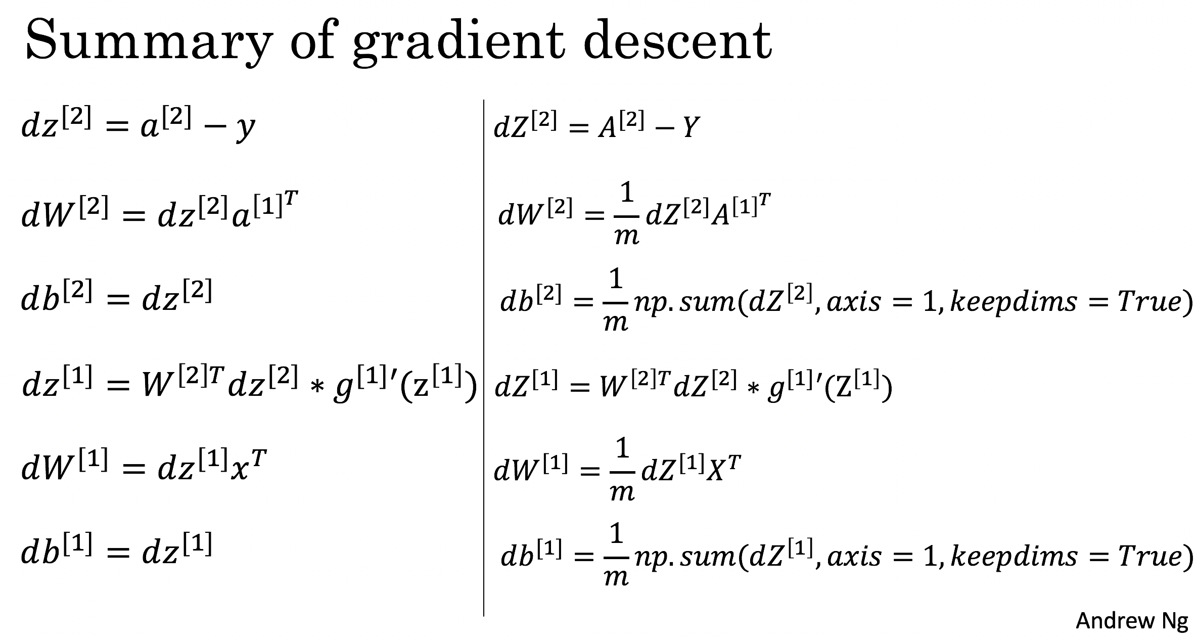
    dZ2 = A2 - Y
    dW2 = 1 / m * np.dot(dZ2, A1.T)
    db2 = 1 / m * np.sum(dZ2, axis = 1, keepdims = True)
    dZ1 = np.dot(W2.T, dZ2) * (1 - np.power(A1, 2))
    dW1 = 1 / m * np.dot(dZ1, X.T)
    db1 = 1 / m * np.sum(dZ1, axis = 1, keepdims = True)
- cost计算
    logprobs = np.multiply(np.log(A2), Y) + np.multiply(np.log(1 - A2), 1 - Y)
    cost = - 1 / m * np.sum(logprobs)
单隐层神经网络代码:
# Package imports
import numpy as np
import matplotlib.pyplot as plt
import sklearn
import sklearn.datasets
import sklearn.linear_model
from planar_utils import plot_decision_boundary, sigmoid, load_planar_dataset, load_extra_datasets

%matplotlib inline

np.random.seed(1) # set a seed so that the results are consistent


def initialize_parameters(n_x, n_h, n_y):
    np.random.seed(2) # we set up a seed so that your output matches ours although the initialization is random.

    W1 = np.random.randn(n_h, n_x) * 0.01
    b1 = np.zeros((n_h, 1))
    W2 = np.random.randn(n_y, n_h)
    b2 = np.zeros((n_y, 1))

    assert (W1.shape == (n_h, n_x))
    assert (b1.shape == (n_h, 1))
    assert (W2.shape == (n_y, n_h))
    assert (b2.shape == (n_y, 1))

    parameters = {"W1": W1,
                  "b1": b1,
                  "W2": W2,
                  "b2": b2}

    return parameters


def forward_propagation(X, parameters):
    # Retrieve each parameter from the dictionary "parameters"
    W1 = parameters["W1"]
    b1 = parameters["b1"]
    W2 = parameters["W2"]
    b2 = parameters["b2"]

    # Implement Forward Propagation to calculate A2 (probabilities)
    Z1 = np.dot(W1, X) + b1
    A1 = np.tanh(Z1)
    Z2 = np.dot(W2, A1) + b2
    A2 = sigmoid(Z2)

    assert(A2.shape == (1, X.shape[1]))

    cache = {"Z1": Z1,
             "A1": A1,
             "Z2": Z2,
             "A2": A2}

    return A2, cache


def compute_cost(A2, Y, parameters):
    m = Y.shape[1] # number of example

    # Compute the cross-entropy cost
    logprobs = np.multiply(np.log(A2), Y) + np.multiply(np.log(1 - A2), 1 - Y)
    cost = - 1 / m * np.sum(logprobs)

    cost = np.squeeze(cost)     # makes sure cost is the dimension we expect.
                                # E.g., turns [[17]] into 17
    assert(isinstance(cost, float))

    return cost


def backward_propagation(parameters, cache, X, Y):
    m = X.shape[1]

    # First, retrieve W1 and W2 from the dictionary "parameters".
    W1 = parameters["W1"]
    W2 = parameters["W2"]

    # Retrieve also A1 and A2 from dictionary "cache".
    A1 = cache["A1"]
    A2 = cache["A2"]

    # Backward propagation: calculate dW1, db1, dW2, db2.
    dZ2 = A2 - Y
    dW2 = 1 / m * np.dot(dZ2, A1.T)
    db2 = 1 / m * np.sum(dZ2, axis = 1, keepdims = True)
    dZ1 = np.dot(W2.T, dZ2) * (1 - np.power(A1, 2))
    dW1 = 1 / m * np.dot(dZ1, X.T)
    db1 = 1 / m * np.sum(dZ1, axis = 1, keepdims = True)

    grads = {"dW1": dW1,
             "db1": db1,
             "dW2": dW2,
             "db2": db2}

    return grads


def update_parameters(parameters, grads, learning_rate = 0.8):
    # Retrieve each parameter from the dictionary "parameters"
    W1 = parameters["W1"]
    b1 = parameters["b1"]
    W2 = parameters["W2"]
    b2 = parameters["b2"]

    # Retrieve each gradient from the dictionary "grads"
    dW1 = grads["dW1"]
    db1 = grads["db1"]
    dW2 = grads["dW2"]
    db2 = grads["db2"]

    # Update rule for each parameter
    W1 = W1 - learning_rate * dW1
    b1 = b1 - learning_rate * db1
    W2 = W2 - learning_rate * dW2
    b2 = b2 - learning_rate * db2

    parameters = {"W1": W1,
                  "b1": b1,
                  "W2": W2,
                  "b2": b2}

    return parameters


def nn_model(X, Y, n_h, num_iterations = 10000, print_cost=False):
    np.random.seed(3)
    n_x = X.shape[0]
    n_y = Y.shape[0]

    # Initialize parameters, then retrieve W1, b1, W2, b2. Inputs: "n_x, n_h, n_y". Outputs = "W1, b1, W2, b2, parameters".
    parameters = initialize_parameters(n_x, n_h, n_y)
    W1 = parameters["W1"]
    b1 = parameters["b1"]
    W2 = parameters["W2"]
    b2 = parameters["b2"]

    # Loop (gradient descent)
    for i in range(0, num_iterations):
        # Forward propagation. Inputs: "X, parameters". Outputs: "A2, cache".
        A2, cache = forward_propagation(X, parameters)

        # Cost function. Inputs: "A2, Y, parameters". Outputs: "cost".
        cost = compute_cost(A2, Y, parameters)

        # Backpropagation. Inputs: "parameters, cache, X, Y". Outputs: "grads".
        grads = backward_propagation(parameters, cache, X, Y)

        # Gradient descent parameter update. Inputs: "parameters, grads". Outputs: "parameters".
        parameters = update_parameters(parameters, grads)

        # Print the cost every 1000 iterations
        if print_cost and i % 1000 == 0:
            print ("Cost after iteration %i: %f" %(i, cost))

    return parameters


def predict(parameters, X):
    # Computes probabilities using forward propagation, and classifies to 0/1 using 0.5 as the threshold.
    A2, cache =  forward_propagation(X, parameters)
    predictions = A2 > 0.5

    return predictions


X, Y = load_planar_dataset()
# Build a model with a n_h-dimensional hidden layer
parameters = nn_model(X, Y, n_h = 4, num_iterations = 10000, print_cost=True)

# Plot the decision boundary
plot_decision_boundary(lambda x: predict(parameters, x.T), X, np.squeeze(Y))
plt.title("Decision Boundary for hidden layer size " + str(4))
# planar_utils.py
import matplotlib.pyplot as plt
import numpy as np
import sklearn
import sklearn.datasets
import sklearn.linear_model

def plot_decision_boundary(model, X, y):
    # Set min and max values and give it some padding
    x_min, x_max = X[0, :].min() - 1, X[0, :].max() + 1
    y_min, y_max = X[1, :].min() - 1, X[1, :].max() + 1
    h = 0.01
    # Generate a grid of points with distance h between them
    # 创造网格,以0.01为间隔划分整个区间
    xx, yy = np.meshgrid(np.arange(x_min, x_max, h), np.arange(y_min, y_max, h))
    # Predict the function value for the whole grid
    # 计算每个网格点上的预测结果
    Z = model(np.c_[xx.ravel(), yy.ravel()])
    # 将预测结果变形为与网格形式一致
    Z = Z.reshape(xx.shape)
    # Plot the contour and training examples
    # xx是x轴值, yy是y轴值, Z是预测结果值, cmap表示采用什么颜色
    plt.contourf(xx, yy, Z, cmap=plt.cm.Spectral) #等位线
    plt.ylabel('x2')
    plt.xlabel('x1')
    plt.scatter(X[0, :], X[1, :], c=y, cmap=plt.cm.Spectral)


def sigmoid(x):
    """
    Compute the sigmoid of x

    Arguments:
    x -- A scalar or numpy array of any size.

    Return:
    s -- sigmoid(x)
    """
    s = 1/(1+np.exp(-x))
    return s

def load_planar_dataset():
    np.random.seed(1)
    m = 400 # number of examples
    N = int(m/2) # number of points per class
    D = 2 # dimensionality
    X = np.zeros((m,D)) # data matrix where each row is a single example
    Y = np.zeros((m,1), dtype='uint8') # labels vector (0 for red, 1 for blue)
    a = 4 # maximum ray of the flower

    for j in range(2):
        ix = range(N*j,N*(j+1))
        t = np.linspace(j*3.12,(j+1)*3.12,N) + np.random.randn(N)*0.2 # theta
        r = a*np.sin(4*t) + np.random.randn(N)*0.2 # radius
        X[ix] = np.c_[r*np.sin(t), r*np.cos(t)]
        Y[ix] = j

    X = X.T
    Y = Y.T

    return X, Y

def load_extra_datasets():
    N = 200
    noisy_circles = sklearn.datasets.make_circles(n_samples=N, factor=.5, noise=.3)
    noisy_moons = sklearn.datasets.make_moons(n_samples=N, noise=.2)
    blobs = sklearn.datasets.make_blobs(n_samples=N, random_state=5, n_features=2, centers=6)
    gaussian_quantiles = sklearn.datasets.make_gaussian_quantiles(mean=None, cov=0.5, n_samples=N, n_features=2, n_classes=2, shuffle=True, random_state=None)
    no_structure = np.random.rand(N, 2), np.random.rand(N, 2)

    return noisy_circles, noisy_moons, blobs, gaussian_quantiles, no_structure

 浙公网安备 33010602011771号