深度学习与Pytorch入门实战(十四)时间序列预测
1. 问题描述
-
已知 [k, k+n)时刻的正弦函数,预测 [k+t, k+n+t)时刻的正弦曲线。
-
因为每个时刻曲线上的点是一个值,即feature_len=1
-
如果给出50个时刻的点,即seq_len=50
-
如果只提供一条曲线供输入,即batch=1
-
输入的shape=[seq_len, batch, feature_len] = [50, 1, 1]。
2. 代码实现
import torch
import torch.nn as nn
import numpy as np
import torch.optim as optim
from matplotlib import pyplot as plt
input_size = 1
batch_size = 1
hidden_size = 16
num_layers = 1
output_size = 1
class Net(nn.Module):
def __init__(self):
super().__init__()
self.rnn = nn.RNN(
input_size=input_size, # feature_len = 1
hidden_size=hidden_size, # 隐藏记忆单元个数hidden_len = 16
num_layers=num_layers, # 网络层数 = 1
batch_first=True # 在传入数据时,按照[batch,seq_len,feature_len]的格式
)
for p in self.rnn.parameters(): # 对RNN层的参数做初始化
nn.init.normal_(p, mean=0.0, std=0.001)
self.linear = nn.Linear(hidden_size, output_size) # 输出层
def forward(self, x, hidden_prev):
"""
x:一次性输入所有样本所有时刻的值(batch,seq_len,feature_len)
hidden_prev:第一个时刻空间上所有层的记忆单元(batch, num_layer, hidden_len)
输出out(batch,seq_len,hidden_len) 和 hidden_prev(batch,num_layer,hidden_len)
"""
out, hidden_prev = self.rnn(x, hidden_prev)
# 因为要把输出传给线性层处理,这里将batch和seq_len维度打平
# 再把batch=1添加到最前面的维度(为了和y做MSE)
# [batch=1,seq_len,hidden_len]->[seq_len,hidden_len]
out = out.view(-1, hidden_size)
#[seq_len,hidden_len]->[seq_len,output_size=1]
out = self.linear(out)
# [seq_len,output_size=1]->[batch=1,seq_len,output_size=1]
out = out.unsqueeze(dim=0)
return out, hidden_prev
# 训练过程
learning_rate = 0.01
model = Net()
criterion = nn.MSELoss()
optimizer = optim.Adam(model.parameters(), lr=learning_rate)
hidden_prev = torch.zeros(batch_size, num_layers, hidden_size) # 初始化记忆单元h0[batch,num_layer,hidden_len]
num_time_steps = 50 # 区间内取多少样本点
for iter in range(6000):
start = np.random.randint(3, size=1)[0] # 在0~3之间随机取开始的时刻点
time_steps = np.linspace(start, start + 10, num_time_steps) # 在[start,start+10]区间均匀地取num_points个点
data = np.sin(time_steps)
data = data.reshape(num_time_step, 1) # [num_time_steps,] -> [num_points,1]
# 输入前49个点(seq_len=49),即下标0~48 [batch, seq_len, feature_len]
x = torch.tensor(data[:-1]).float().view(1, num_time_steps - 1, 1)
# 预测后49个点,即下标1~49
y = torch.tensor(data[1:]).float().view(1, num_time_steps - 1, 1)
# 以上步骤生成(x,y)数据对
output, hidden_prev = model(x, hidden_prev) # 喂入模型得到输出
hidden_prev = hidden_prev.detach() # at
loss = criterion(output, y) # 计算MSE损失
model.zero_grad()
loss.backward()
optimizer.step()
if iter % 1000 == 0:
print("Iteration: {} loss {}".format(iter, loss.item()))
# 测试过程
# 先用同样的方式生成一组数据x,y
start = np.random.randint(3, size=1)[0]
time_steps = np.linspace(start, start + 10, num_time_steps)
data = np.sin(time_steps)
data = data.reshape(num_time_steps, 1)
x = torch.tensor(data[:-1]).float().view(1, num_time_steps - 1, 1)
y = torch.tensor(data[1:]).float().view(1, num_time_steps - 1, 1)
predictions = []
input = x[:, 0, :] # 取seq_len里面第0号数据
input = input.view(1, 1, 1) # input:[1,1,1]
for _ in range(x.shape[1]): # 迭代seq_len次
pred, hidden_prev = model(input, hidden_prev)
input = pred # 预测出的(下一个点的)序列pred当成输入(或者直接写成input, hidden_prev = model(input, hidden_prev))
predictions.append(pred.detach().numpy().ravel()[0])
x = x.data.numpy()
y = y.data.numpy()
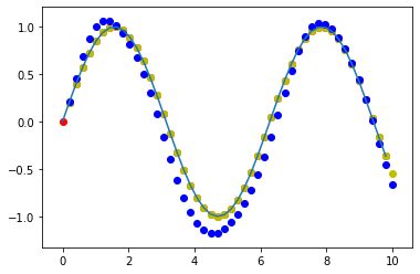
plt.plot(time_steps[:-1], x.ravel())
plt.scatter(time_steps[:-1], x.ravel(), c='r') # x值
plt.scatter(time_steps[1:], y.ravel(), c='y') # y值
plt.scatter(time_steps[1:], predictions, c='b') # y的预测值
plt.show()
Iteration: 0 loss 0.47239747643470764
Iteration: 1000 loss 0.0028104630764573812
Iteration: 2000 loss 0.00022502802312374115
Iteration: 3000 loss 0.00013326731277629733
Iteration: 4000 loss 0.00011971688218181953
Iteration: 5000 loss 0.00046832612133584917
3. 梯度裁剪
如果发生梯度爆炸,在上面代码loss.backward() 与 optimizer.step() 之间要进行梯度裁剪:
    model.zero_grad()
    loss.backward()
    # 梯度裁剪
    for p in model.parameters():
        # print(p.grad.norm())                 # 查看参数p的梯度
        torch.nn.utils.clip_grad_norm_(p, 10)  # 将梯度裁剪到小于10
    optimizer.step()

 浙公网安备 33010602011771号