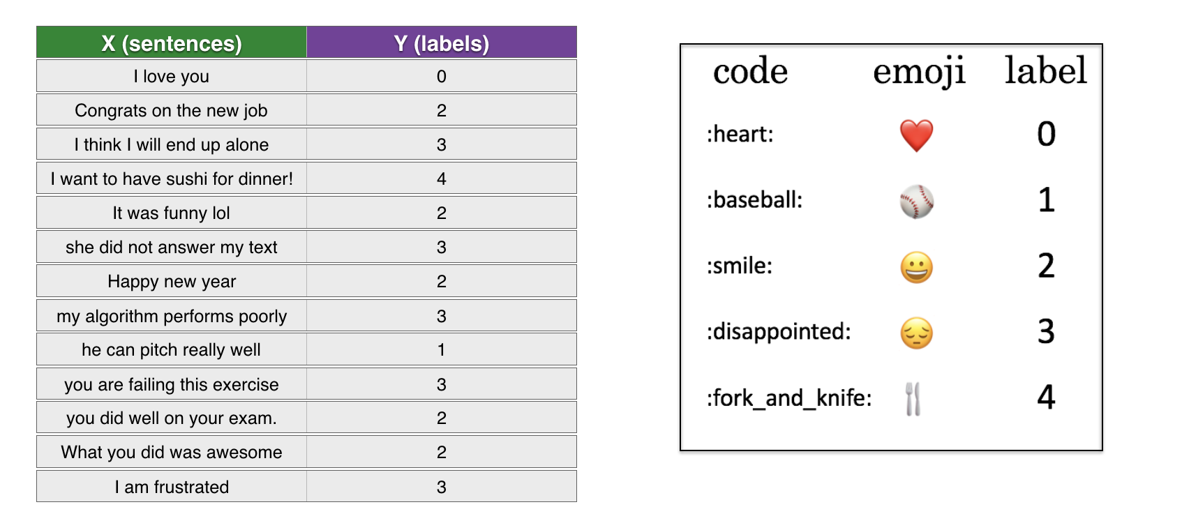
Sequence Model-week2编程题2-Emoji表情生成器
1. Emoji表情生成器
下面,我们要使用词向量(word vector)来构建一个表情生成器。
- 你将实现一个模型:输入一句话 (如 "Let's go see the baseball game tonight!") 然后找到使用在这句话上最合适的表情(⚾️).
使用单词向量来改进表情符号查找
-
在许多表情符号界面中,你需要记住,❤是“heart”符号,而不是“love”符号。
- 换句话说,你必须记住输入“heart”来找到想要的表情符号,而输入“love”不会带来这个符号。
-
我们可以使用文字向量来制作更灵活的表情符号接口!
-
当使用单词向量时,您将看到,即使您的训练集显式地将几个单词与特定的表情符号关联起来,您的算法也将能够将测试集中的额外单词泛化并关联到相同的表情符号。
-
即使这些额外的单词甚至没有出现在训练集中,这也是有效的。
-
这允许您构建从句子到表情符号的精确分类器映射,甚至使用一个小的训练集。
-
需要实现的:
-
你将从使用 word embeddings 的 baseline model(Emojifier-V1) 开始。
-
然后,你将构建一个更加复杂的模型(Emojifier-V2),该模型进一步结合了LSTM。
1.1 导入包
import numpy as np
from emo_utils import *
import emoji
import matplotlib.pyplot as plt

%matplotlib inline
2. 基础模型(Baseline model: Emojifier-V1)
2.1 数据集(Dataset EMOJISET)
我们来构建一个简单的分类器,首先是数据集(X,Y):
-
X:包含了127个字符串类型的短句
-
Y:包含一个0到4之间的整数标签,对应于每个句子的表情符号
导入数据集,127个训练集样本,56个测试集样本 (???输出明明是132个训练样本)
X_train, Y_train = read_csv('data/train_emoji.csv')
X_test, Y_test = read_csv('data/tesss.csv')

print(X_train.shape, Y_train.shape)
print(X_test.shape, Y_test.shape)
(132,) (132,)
(56,) (56,)
print(max(X_train, key=len).split())
print(len(max(X_train, key=len).split()))   # 最长句子的单词长度

maxLen = len(max(X_train, key=len).split())
['I', 'am', 'so', 'impressed', 'by', 'your', 'dedication', 'to', 'this', 'project']
10
运行以下单元格,从 X_train 打印句子,从 Y_train 打印相应的标签。
- 更改
idx来查看不同的示例.
for idx in range(10):
    print(X_train[idx], label_to_emoji(Y_train[idx]))
never talk to me again 😞
I am proud of your achievements 😄
It is the worst day in my life 😞
Miss you so much ❤️
food is life 🍴
I love you mum ❤️
Stop saying bullshit 😞
congratulations on your acceptance 😄
The assignment is too long 😞
I want to go play ⚾
2.2 Emojifier-V1概述
实现一个叫“Emojifier-V1”的基准模型。
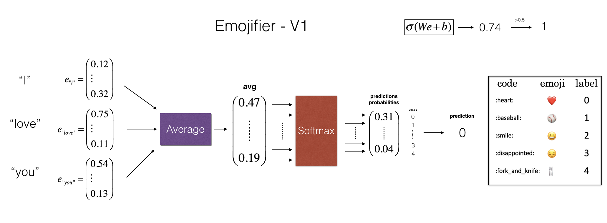
Inputs and outputs
-
模型的输入是一个句子对应的字符串 (e.g. "I love you).
-
模型的输出是维度为(1,5) 的概率向量 (there are 5 emojis to choose from).
-
将维度(1,5)的概率向量 传递给 argmax 层,该层提取概率最高的表情符号的索引。
One-hot encoding
-
为了使得我们的标签成为一种适合于训练 softmax分类器的格式,将 Y 当前维度(m, 1) 转换成 "one-hot representation" (m,5)
-
每行都是一个 one-hot向量,给出一个示例的标签。
-
这里,
Y_oh在Y_oh_train和Y_oh_test的变量名中的代表 "Y-one-hot"。
-
Y_oh_train = convert_to_one_hot(Y_train, C = 5)   # 因为有5种输出
Y_oh_test = convert_to_one_hot(Y_test, C = 5)

print(Y_oh_train[:10])
print(Y_train.shape)
print(Y_oh_train.shape)
[[0. 0. 0. 1. 0.]
 [0. 0. 1. 0. 0.]
 [0. 0. 0. 1. 0.]
 [1. 0. 0. 0. 0.]
 [0. 0. 0. 0. 1.]
 [1. 0. 0. 0. 0.]
 [0. 0. 0. 1. 0.]
 [0. 0. 1. 0. 0.]
 [0. 0. 0. 1. 0.]
 [0. 1. 0. 0. 0.]]
(132,)
(132, 5)
观察 convert_to_one_hot()实现的:
idx = 50
# print(f"Sentence '{X_train[50]}' has label index {Y_train[idx]}, which is emoji {label_to_emoji(Y_train[idx])}")  # python3.7写法
# print(f"Label index {Y_train[idx]} in one-hot encoding format is {Y_oh_train[idx]}")

print(X_train[idx], Y_train[idx], label_to_emoji(Y_train[idx]))
print(Y_train[index], "is converted into one hot", Y_oh_train[index])
I missed you 0 ❤️
0 is converted into one hot [1. 0. 0. 0. 0.]
2.3 实现 Emojifier-V1
如上图所示,第一步:
-
将输入句中的每个单词转换为它们的词向量表示。
-
然后,取单词向量的平均值。
-
与先前的练习类似,我们将使用 预训练的50维GloVe词嵌入。
已导入:
word_to_index:从 词汇 映射到 词汇索引 的字典。- (400,001 words, 有效索引从 0 到 400,000)
index_to_word: 从 索引 映射到 它们相应词汇 的字典。word_to_vec_map: 字典将 单词 映射到 它们的GloVe向量表示。
word = "cucumber"
idx = 289846
print("the index of", word, "in the vocabulary is", word_to_index[word])
print("the", str(idx) + "th word in the vocabulary is", index_to_word[idx])
the index of cucumber in the vocabulary is 113317
the 289846th word in the vocabulary is potatos
Exercise: 实现sentence_to_avg(),需要进行下面两步:
- 将每个句子转换成小写,然后把句子分成一个单词列表、
X.lower()andX.split()might be useful.
- 对句子中的每个单词,访问其 GloVe表示。
- 然后取所有这些 词向量 的平均值
- 可以使用
numpy.zeros().
Additional Hints
- 当创建
avg零数组时,你将希望它是与word_to_vec_map中其他单词向量相同维度的 向量.- 你可以选择一个在
word_to_vec_map中的单词,并访问其.shape字段。
- 你可以选择一个在
# GRADED FUNCTION: sentence_to_avg

def sentence_to_avg(sentence, word_to_vec_map):
    """
    Converts a sentence (string) into a list of words (strings). Extracts the GloVe representation of each word
    and averages its value into a single vector encoding the meaning of the sentence.

    Arguments:
    sentence -- string, one training example from X
    word_to_vec_map -- dictionary mapping every word in a vocabulary into its 50-dimensional vector representation

    Returns:
    avg -- average vector encoding information about the sentence, numpy-array of shape (50,)
    """

    ### START CODE HERE ###
    # Step 1: Split sentence into list of lower case words (≈ 1 line)
    words = sentence.lower().split()

    # Initialize the average word vector, should have the same shape as your word vectors.
    avg = np.zeros(len(words))

    # Step 2: average the word vectors. You can loop over the words in the list "words".
    total = 0
    for w in words:
        total += word_to_vec_map[w]
    avg = total / len(words)

    ### END CODE HERE ###

    return avg
测试:
avg = sentence_to_avg("Morrocan couscous is my favorite dish", word_to_vec_map)
print("avg = \n", avg)
avg =
 [-0.008005    0.56370833 -0.50427333  0.258865    0.55131103  0.03104983
 -0.21013718  0.16893933 -0.09590267  0.141784   -0.15708967  0.18525867
  0.6495785   0.38371117  0.21102167  0.11301667  0.02613967  0.26037767
  0.05820667 -0.01578167 -0.12078833 -0.02471267  0.4128455   0.5152061
  0.38756167 -0.898661   -0.535145    0.33501167  0.68806933 -0.2156265
  1.797155    0.10476933 -0.36775333  0.750785    0.10282583  0.348925
 -0.27262833  0.66768    -0.10706167 -0.283635    0.59580117  0.28747333
 -0.3366635   0.23393817  0.34349183  0.178405    0.1166155  -0.076433
  0.1445417   0.09808667]
Model
model()所有部分已经实现。
使用 sentence_to_avg() 后需要:
- 通过前向传播传递平均数
- 计算cost
- 反向传播更新 softmax 参数
Exercise: 实现 model().
- 你要在前向传播实现的方程 和 计算cross-entropy:
- 变量 \(Y_{oh}\) ("Y one hot") 是输出标签的 one-hot encoding。
Note 可以提出更有效的向量化实现,现在,我们使用for循环,更好的理解,并容易调试.
# GRADED FUNCTION: model

def model(X, Y, word_to_vec_map, learning_rate = 0.01, num_iterations = 400):
    """
    Model to train word vector representations in numpy.

    Arguments:
    X -- input data, numpy array of sentences as strings, of shape (m, 1)
    Y -- labels, numpy array of integers between 0 and 7, numpy-array of shape (m, 1)
    word_to_vec_map -- dictionary mapping every word in a vocabulary into its 50-dimensional vector representation
    learning_rate -- learning_rate for the stochastic gradient descent algorithm
    num_iterations -- number of iterations

    Returns:
    pred -- vector of predictions, numpy-array of shape (m, 1)
    W -- weight matrix of the softmax layer, of shape (n_y, n_h)
    b -- bias of the softmax layer, of shape (n_y,)
    """

    np.random.seed(1)

    # Define number of training examples
    m = Y.shape[0]                          # number of training examples
    n_y = 5                                 # number of classes
    n_h = 50                                # dimensions of the GloVe vectors

    # Initialize parameters using Xavier initialization
    W = np.random.randn(n_y, n_h) / np.sqrt(n_h)
    b = np.zeros((n_y,))

    # Convert Y to Y_onehot with n_y classes
    Y_oh = convert_to_one_hot(Y, C = n_y)

    # Optimization loop
    for t in range(num_iterations): # Loop over the number of iterations
        for i in range(m):          # Loop over the training examples

            ### START CODE HERE ### (≈ 4 lines of code)
            # Average the word vectors of the words from the i'th training example
            avg = sentence_to_avg(X[i], word_to_vec_map)

            # Forward propagate the avg through the softmax layer
            z = np.dot(W, avg) + b
            a = softmax(z)

            # Compute cost using the i'th training label's one hot representation and "A" (the output of the softmax)
            cost = - np.sum(Y_oh * np.log(a))
            ### END CODE HERE ###

            # Compute gradients
            dz = a - Y_oh[i]
            dW = np.dot(dz.reshape(n_y,1), avg.reshape(1, n_h))
            db = dz

            # Update parameters with Stochastic Gradient Descent
            W = W - learning_rate * dW
            b = b - learning_rate * db

        if t % 100 == 0:
            print("Epoch: " + str(t) + " --- cost = " + str(cost))
            pred = predict(X, Y, W, b, word_to_vec_map) #predict is defined in emo_utils.py

    return pred, W, b
print(X_train.shape)
print(Y_train.shape)
print(np.eye(5)[Y_train.reshape(-1)].shape)
print(X_train[0])
print(type(X_train))
Y = np.asarray([5,0,0,5, 4, 4, 4, 6, 6, 4, 1, 1, 5, 6, 6, 3, 6, 3, 4, 4])
print(Y.shape)

X = np.asarray(['I am going to the bar tonight', 'I love you', 'miss you my dear',
 'Lets go party and drinks','Congrats on the new job','Congratulations',
 'I am so happy for you', 'Why are you feeling bad', 'What is wrong with you',
 'You totally deserve this prize', 'Let us go play football',
 'Are you down for football this afternoon', 'Work hard play harder',
 'It is suprising how people can be dumb sometimes',
 'I am very disappointed','It is the best day in my life',
 'I think I will end up alone','My life is so boring','Good job',
 'Great so awesome'])

print(X.shape)
print(np.eye(5)[Y_train.reshape(-1)].shape)
print(type(X_train))
(132,)
(132,)
(132, 5)
never talk to me again
<class 'numpy.ndarray'>
(20,)
(20,)
(132, 5)
<class 'numpy.ndarray'>
pred, W, b = model(X_train, Y_train, word_to_vec_map)
print(pred)
Epoch: 0 --- cost = 227.52718163332128
Accuracy: 0.3484848484848485
Epoch: 100 --- cost = 418.19864120233854
Accuracy: 0.9318181818181818
Epoch: 200 --- cost = 482.72727709506074
Accuracy: 0.9545454545454546
Epoch: 300 --- cost = 516.6590639612792
Accuracy: 0.9696969696969697
[[3.]
 [2.]
 [3.]
 [0.]
 [4.]
 [0.]
 [3.]
 [2.]
 [3.]
 [1.]
 [3.]
 [3.]
 [1.]
 [3.]
 [2.]
 [3.]
 [2.]
 [3.]
 [1.]
 [2.]
 [3.]
 [0.]
 [2.]
 [2.]
 [2.]
 [1.]
 [4.]
 [3.]
 [3.]
 [4.]
 [0.]
 [3.]
 [4.]
 [2.]
 [0.]
 [3.]
 [2.]
 [2.]
 [3.]
 [4.]
 [2.]
 [2.]
 [0.]
 [2.]
 [3.]
 [0.]
 [3.]
 [2.]
 [4.]
 [3.]
 [0.]
 [3.]
 [3.]
 [3.]
 [4.]
 [2.]
 [1.]
 [1.]
 [1.]
 [2.]
 [3.]
 [1.]
 [0.]
 [0.]
 [0.]
 [3.]
 [4.]
 [4.]
 [2.]
 [2.]
 [1.]
 [2.]
 [0.]
 [3.]
 [2.]
 [2.]
 [0.]
 [3.]
 [3.]
 [1.]
 [2.]
 [1.]
 [2.]
 [2.]
 [4.]
 [3.]
 [3.]
 [2.]
 [4.]
 [0.]
 [0.]
 [3.]
 [3.]
 [3.]
 [3.]
 [2.]
 [0.]
 [1.]
 [2.]
 [3.]
 [0.]
 [2.]
 [2.]
 [2.]
 [3.]
 [2.]
 [2.]
 [2.]
 [4.]
 [1.]
 [1.]
 [3.]
 [3.]
 [4.]
 [1.]
 [2.]
 [1.]
 [1.]
 [3.]
 [1.]
 [0.]
 [4.]
 [0.]
 [3.]
 [3.]
 [4.]
 [4.]
 [1.]
 [4.]
 [3.]
 [0.]
 [2.]]
2.4 Examining test set performance
print("Training set:")
pred_train = predict(X_train, Y_train, W, b, word_to_vec_map)
print('Test set:')
pred_test = predict(X_test, Y_test, W, b, word_to_vec_map)
Training set:
Accuracy: 0.9772727272727273
Test set:
Accuracy: 0.8571428571428571
The model matches emojis to relevant words
In the training set, the algorithm saw the sentence
"I love you"
with the label ❤️.
- You can check that the word "adore" does not appear in the training set.
- Nonetheless, lets see what happens if you write "I adore you."
X_my_sentences = np.array(["i adore you", "i love you", "funny lol", "lets play with a ball", "food is ready", "not feeling happy"])
Y_my_labels = np.array([[0], [0], [2], [1], [4],[3]])

pred = predict(X_my_sentences, Y_my_labels , W, b, word_to_vec_map)
print_predictions(X_my_sentences, pred)
Accuracy: 0.8333333333333334
i adore you ❤️
i love you ❤️
funny lol 😄
lets play with a ball ⚾
food is ready 🍴
not feeling happy 😄
模型中不考虑单词排序
- 注意,模型没有正确地理解以下句子:
"not feeling happy"
这个算法忽略了单词排序,所以不善于理解“不快乐”之类的短语;
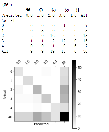
混淆矩阵
-
打印混淆矩阵也有助于理解,哪些classes对你的模型更困难。
-
混淆矩阵 显示标签为一个类("actual" class)的示例 被("predicted" class)不同类的算法 错误标记的频率。
print(Y_test.shape)
print('           '+ label_to_emoji(0)+ '    ' + label_to_emoji(1) + '    ' +  label_to_emoji(2)+ '    ' + label_to_emoji(3)+'   ' + label_to_emoji(4))
print(pd.crosstab(Y_test, pred_test.reshape(56,), rownames=['Actual'], colnames=['Predicted'], margins=True))
plot_confusion_matrix(Y_test, pred_test)
3. Emojifier-V2: Using LSTMs in Keras
构建一个LSTM模型,它以 word sequences 作为输入
-
model将能够解释 单词排序
-
Emojifier-V2将继续使用 预先训练过的单词嵌入 来表示单词。
-
将 词嵌入 放入 LSTM
-
LSTM 将学会预测最合适的 表情符号
运行下面代码:
import numpy as np
np.random.seed(0)
from keras.models import Model
from keras.layers import Dense, Input, Dropout, LSTM, Activation
from keras.layers.embeddings import Embedding
from keras.preprocessing import sequence
from keras.initializers import glorot_uniform
np.random.seed(1)
3.1 模型概述
Emojifier-v2结构:

3.2 Keras and mini-batching
-
这里,将使用
mini-batch训练Keras -
但是大部分深度学习框架 要求同样的mini-batch中 所有sequences具有 相同的长度的文字
- 这就是允许向量化工作的原因:如果你有一个3字的句子和一个4字的句子,那么它们所需的计算是不同的(一个需要3个LSTM,一个需要4个LSTM),所以不可能同时做它们。
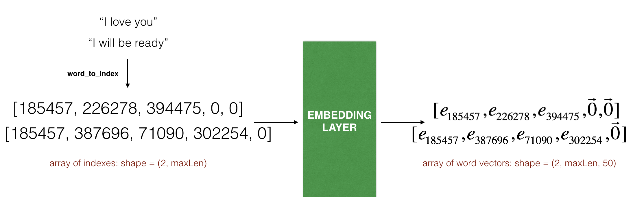
填补(Paddding)处理不同长度的sequences
-
设置最大序列长度
-
填补所有序列,使之具有相同的长度
填充的例子
-
给定序列的最大长度为20,我们可以用“0”填充每个句子,使每个输入句子长度为20.
-
因此,“I love you”这句话可以被表示为 \((e_{I}, e_{love}, e_{you}, \vec{0}, \vec{0}, \ldots, \vec{0})\).
-
在这个例子中,任何超过20个字的句子都必须被截断.
-
选择最大序列长度的一种方法是:在训练集中,选择最长句子的长度.
3.3 The Embedding layer
-
在Keras中,嵌入矩阵(Embedding Matrix) 表示为“layer”
-
嵌入矩阵(Embedding Matrix) 映射单词索引 到 嵌入向量(Embedding vectors)
-
单词索引 是正整数
-
嵌入向量是固定大小的dense vectors
-
当我们说向量是“dense”时,在这种情况下,这意味着 大多数值都是非零的。 作为一个反例,一个one-hot向量不是“dense”
-
-
嵌入矩阵可以两种方式推导出:
-
训练模型从 随意值 开始推导 embedding
-
使用预先训练的 embedding
-
使用和更新预先训练的嵌入
-
在本部分,您将学习如何在Keras中创建 Embedding层
-
你将用 GloVe 50-dimensional vectors 初始化 Embedding layer
-
下面展示keras 如何允许你 训练或离开 固定层
- 因为我们训练集很小,我们将把 GloVe embedding固定下来,而不是更新它
输入 和 输出到embedding layer
-
Embedding()layer 的 输入 是一个维度为 (batch size, max input length) 的整数矩阵-
此输入 对应于 转换为索引列表(整数)的句子.
-
输入中最大的整数(最高的单词索引) 应该不大于词汇表的长度。
-
-
The embedding layer 输出 数组维度为 (batch size, max input length, dimension of word vectors).
-
下图展示了两个例句通过 embedding layer 的传播.
-
两个例子都被 填补0 到
max_len=5的长度. -
The word embeddings 的长度为 50 units.
-
表示的最终维度是
(2, max_len, 50).
-
准备输入句子
Exercise:
- 实现
sentences_to_indices, 处理一组 sentences (x) 并将输入返回到 embedding layer:-
将每个训练句子转换成一个索引列表(索引对应于句子中的每个单词)
-
用0填充这些列表,使得它们的长度是最长句子的长度。
-
for idx, val in enumerate(["I", "like", "learning"]):
    print(idx, val)
0 I
1 like
2 learning
# GRADED FUNCTION: sentences_to_indices

def sentences_to_indices(X, word_to_index, max_len):
    """
    Converts an array of sentences (strings) into an array of indices corresponding to words in the sentences.
    The output shape should be such that it can be given to `Embedding()` (described in Figure 4).

    Arguments:
    X -- array of sentences (strings), of shape (m, 1)
    word_to_index -- a dictionary containing the each word mapped to its index
    max_len -- maximum number of words in a sentence. You can assume every sentence in X is no longer than this.

    Returns:
    X_indices -- array of indices corresponding to words in the sentences from X, of shape (m, max_len)
    """

    m = X.shape[0]                                   # number of training examples

    ### START CODE HERE ###
    # Initialize X_indices as a numpy matrix of zeros and the correct shape (≈ 1 line)
    X_indices = np.zeros([m, max_len])

    for i in range(m):                               # loop over training examples 所有句子

        # Convert the ith training sentence in lower case and split is into words. You should get a list of words.
        sentence_words = X[i].lower().split()

        # Initialize j to 0
        j = 0

        # Loop over the words of sentence_words  一个句子的每个单词
        for w in sentence_words:
            # Set the (i,j)th entry of X_indices to the index of the correct word.
            X_indices[i, j] = word_to_index[w]  # 不够的长度上,有0
            # Increment j to j + 1
            j = j + 1

    ### END CODE HERE ###

    return X_indices
测试
X1 = np.array(["funny lol", "lets play baseball", "food is ready for you"])
X1_indices = sentences_to_indices(X1,word_to_index, max_len = 5)
print("X1 =", X1)
print("X1_indices =\n", X1_indices)
X1 = ['funny lol' 'lets play baseball' 'food is ready for you']
X1_indices =
 [[155345. 225122.      0.      0.      0.]
 [220930. 286375.  69714.      0.      0.]
 [151204. 192973. 302254. 151349. 394475.]]
Build embedding layer
现在我们就在Keras中构建Embedding()层,我们使用的是已经训练好了的词向量,在构建之后,使用sentences_to_indices()生成的数据作为输入,Embedding()层将返回每个句子的词嵌入。
Exercise: 实现 pretrained_embedding_layer() with these steps:
-
将 embedding matrix 初始化为零的numpy数组
-
嵌入矩阵(embedding matrix)对词汇表中的每个唯一单词都有一行。
- 有一个额外的行来处理 “unknown” 单词,所以
vocab_len是 唯一词数量 + 1
- 有一个额外的行来处理 “unknown” 单词,所以
-
每行将存储一个单词的向量表示
- 例如,如果使用GloVe字向量,一行可能有50个位置长。
-
emb_dim表示 word embedding 的长度
-
-
使用
word_to_vec_map来将 词嵌入(word embeddings)向量 填充到嵌入矩阵(embedding matrix)的每一行-
word_to_index中的每个单词是 一个字符串 -
word_to_vec_map是一个字典,其中key是字符串,value是单词向量
-
-
定义 Keras 的 embedding layer
-
使用 Embedding().
-
输入维度 等于 词汇表长度(number of unique words plus one).
-
输出维度 等于 在词嵌入中 等于 词嵌入的长度(number of positions).
-
设置
trainable = False,确保这层不会被训练, 然后它将不允许 optimization algorithm 修改词嵌入的值
-
-
设置 embedding weights 等于 embedding matrix.
# GRADED FUNCTION: pretrained_embedding_layer

def pretrained_embedding_layer(word_to_vec_map, word_to_index):
    """
    Creates a Keras Embedding() layer and loads in pre-trained GloVe 50-dimensional vectors.

    Arguments:
    word_to_vec_map -- dictionary mapping words to their GloVe vector representation.
    word_to_index -- dictionary mapping from words to their indices in the vocabulary (400,001 words)

    Returns:
    embedding_layer -- pretrained layer Keras instance
    """

    vocab_len = len(word_to_index) + 1                  # adding 1 to fit Keras embedding (requirement)
    emb_dim = word_to_vec_map["cucumber"].shape[0]      # define dimensionality of your GloVe word vectors (= 50)

    ### START CODE HERE ###
    # Step 1
    # Initialize the embedding matrix as a numpy array of zeros.
    # See instructions above to choose the correct shape.
    emb_matrix = np.zeros([vocab_len, emb_dim])

    # Step 2
    # Set each row "idx" of the embedding matrix to be
    # the word vector representation of the idx'th word of the vocabulary
    for word, idx in word_to_index.items():
        emb_matrix[idx, :] = word_to_vec_map[word]

    # Step 3
    # Define Keras embedding layer with the correct input and output sizes
    # Make it non-trainable.
    embedding_layer = Embedding(vocab_len, emb_dim, trainable=False)
    ### END CODE HERE ###

    # Step 4 (already done for you; please do not modify)
    # Build the embedding layer, it is required before setting the weights of the embedding layer.
    embedding_layer.build((None,)) # Do not modify the "None".  This line of code is complete as-is.

    # Set the weights of the embedding layer to the embedding matrix. Your layer is now pretrained.
    embedding_layer.set_weights([emb_matrix])

    return embedding_layer
embedding_layer = pretrained_embedding_layer(word_to_vec_map, word_to_index)
print("weights[0][1][3] =", embedding_layer.get_weights()[0][1][3])
weights[0][1][3] = -0.3403
3.3 Building the Emojifier-V2
现在构建 Emojifier-V2 model,你需要 feed the embedding layer's output to an LSTM network.
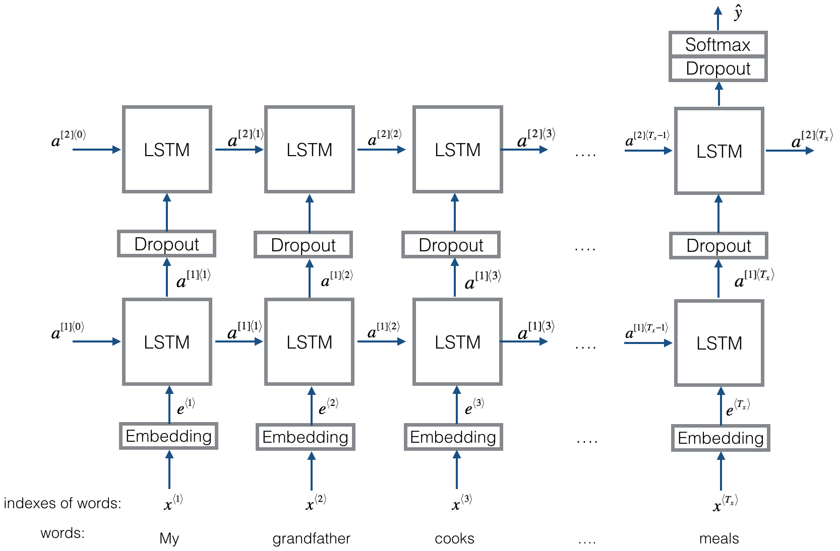
Exercise: 实现 Emojify_V2(), 构建上图 keras的结构
-
模型输入是 一个维度为 (
m,max_len, ) 的 array of sentences,定义为input_shape. -
模型输出是 一个维度为 (
m,C = 5) 的 softmax 可能性向量(probability vector). -
You may need to use the following Keras layers:
- Input()
- Set the
shapeanddtypeparameters. - The inputs are integers, so you can specify the data type as a string, 'int32'.
- Set the
- LSTM()
- Set the
unitsandreturn_sequencesparameters.
- Set the
- Dropout()
- Set the
rateparameter.
- Set the
- Dense()
- Set the
units, - Note that
Dense()has anactivationparameter. For the purposes of passing the autograder, please do not set the activation withinDense(). Use the separateActivationlayer to do so.
- Set the
- Activation().
- You can pass in the activation of your choice as a lowercase string.
- Model
Setinputsandoutputs.
- Input()
Additional Hints
- 记住这些 Keras layers return an object, 你需要将前一层的输出作为输入参数放到这个object。
# How to use Keras layers in two lines of code
dense_object = Dense(units = ...)
X = dense_object(inputs)

# How to use Keras layers in one line of code
X = Dense(units = ...)(inputs)
-
The
embedding_layerthat is returned bypretrained_embedding_layeris a layer object that can be called as a function, passing in a single argument (sentence indices). -
Here is some sample code in case you're stuck
raw_inputs = Input(shape=(maxLen,), dtype='int32')
preprocessed_inputs = ... # some pre-processing
X = LSTM(units = ..., return_sequences= ...)(processed_inputs)
X = Dropout(rate = ..., )(X)
...
X = Dense(units = ...)(X)
X = Activation(...)(X)
model = Model(inputs=..., outputs=...)
...
# GRADED FUNCTION: Emojify_V2

def Emojify_V2(input_shape, word_to_vec_map, word_to_index):
    """
    Function creating the Emojify-v2 model's graph.

    Arguments:
    input_shape -- shape of the input, usually (max_len,)
    word_to_vec_map -- dictionary mapping every word in a vocabulary into its 50-dimensional vector representation
    word_to_index -- dictionary mapping from words to their indices in the vocabulary (400,001 words)

    Returns:
    model -- a model instance in Keras
    """

    ### START CODE HERE ###
    # Define sentence_indices as the input of the graph.
    # It should be of shape input_shape and dtype 'int32' (as it contains indices, which are integers).
    sentence_indices = Input(shape=input_shape, dtype='int32')   # (m, max_len)

    # Create the embedding layer pretrained with GloVe Vectors (≈1 line)
    embedding_layer = pretrained_embedding_layer(word_to_vec_map, word_to_index)

    # Propagate sentence_indices through your embedding layer
    # (See additional hints in the instructions).
    embeddings = embedding_layer(sentence_indices)

    # Propagate the embeddings through an LSTM layer with 128-dimensional hidden state
    # The returned output should be a batch of sequences.
    X = LSTM(units=128, return_sequences=True)(embeddings)
    # Add dropout with a probability of 0.5
    X = Dropout(rate=0.5)(X)
    # Propagate X trough another LSTM layer with 128-dimensional hidden state
    # The returned output should be a single hidden state, not a batch of sequences.
    X = LSTM(units=128, return_sequences=False)(X)
    # Add dropout with a probability of 0.5
    X = Dropout(rate=0.5)(X)
    # Propagate X through a Dense layer with 5 units
    X = Dense(5, activation='softmax')(X)
    # Add a softmax activation
    X = Activation('softmax')(X)

    # Create Model instance which converts sentence_indices into X.
    model = Model(inputs=sentence_indices, outputs=X)

    ### END CODE HERE ###

    return model
model = Emojify_V2((maxLen,), word_to_vec_map, word_to_index)
model.summary()
Because all sentences in the dataset are less than 10 words, we chose max_len = 10. You should see your architecture, it uses "20,223,927" parameters, of which 20,000,050 (the word embeddings) are non-trainable, and the remaining 223,877 are. Because our vocabulary size has 400,001 words (with valid indices from 0 to 400,000) there are 400,001*50 = 20,000,050 non-trainable parameters.(词嵌入为50长度的)
_________________________________________________________________
Layer (type)                 Output Shape              Param #
=================================================================
input_1 (InputLayer)         (None, 10)                0
_________________________________________________________________
embedding_2 (Embedding)      (None, 10, 50)            20000050
_________________________________________________________________
lstm_1 (LSTM)                (None, 10, 128)           91648
_________________________________________________________________
dropout_1 (Dropout)          (None, 10, 128)           0
_________________________________________________________________
lstm_2 (LSTM)                (None, 128)               131584
_________________________________________________________________
dropout_2 (Dropout)          (None, 128)               0
_________________________________________________________________
dense_1 (Dense)              (None, 5)                 645
_________________________________________________________________
activation_1 (Activation)    (None, 5)                 0
=================================================================
Total params: 20,223,927
Trainable params: 223,877
Non-trainable params: 20,000,050
_________________________________________________________________
编译模型,需要定义 loss, optimizer and metrics your are want to use. 使用 categorical_crossentropy loss, adam optimizer and ['accuracy'] metrics 编译你的模型:
model.compile(loss='categorical_crossentropy', optimizer='adam', metrics=['accuracy'])
训练模型,输入为 维度(m, max_len)的数组,输出为 维度(m, number of classed)。因此,需要将 X_train(句子array) 转换为 X_train_indices(句子的word indices列表),Y_train(indices标签) 转换为 Y_train_oh(one-hot向量标签)
X_train_indices = sentences_to_indices(X_train, word_to_index, maxLen)
Y_train_oh = convert_to_one_hot(Y_train, C = 5)
print(X_train.shape, X_train_indices.shape)
print(Y_train.shape, Y_train_oh.shape)
(132,) (132, 10)
(132,) (132, 5)
迭代50次,batch-size为32,训练数据
model.fit(X_train_indices, Y_train_oh, epochs = 50, batch_size = 32, shuffle=True)
Epoch 1/50
132/132 [==============================] - 2s - loss: 1.6044 - acc: 0.2500
Epoch 2/50
132/132 [==============================] - 0s - loss: 1.5841 - acc: 0.2727
Epoch 3/50
132/132 [==============================] - 0s - loss: 1.5600 - acc: 0.3333
Epoch 4/50
132/132 [==============================] - 0s - loss: 1.5559 - acc: 0.2955
Epoch 5/50
132/132 [==============================] - 0s - loss: 1.5283 - acc: 0.3409
Epoch 6/50
132/132 [==============================] - 0s - loss: 1.5262 - acc: 0.3788
Epoch 7/50
132/132 [==============================] - 0s - loss: 1.4912 - acc: 0.4470
Epoch 8/50
132/132 [==============================] - 0s - loss: 1.4346 - acc: 0.5152
Epoch 9/50
132/132 [==============================] - 0s - loss: 1.3812 - acc: 0.5530
Epoch 10/50
132/132 [==============================] - 0s - loss: 1.3932 - acc: 0.5227
Epoch 11/50
132/132 [==============================] - 0s - loss: 1.3193 - acc: 0.6136
Epoch 12/50
132/132 [==============================] - 0s - loss: 1.2492 - acc: 0.6818
Epoch 13/50
132/132 [==============================] - 0s - loss: 1.2639 - acc: 0.7121
Epoch 14/50
132/132 [==============================] - 0s - loss: 1.1712 - acc: 0.7879
Epoch 15/50
132/132 [==============================] - 0s - loss: 1.1392 - acc: 0.8258
Epoch 16/50
132/132 [==============================] - 0s - loss: 1.1134 - acc: 0.8258
Epoch 17/50
132/132 [==============================] - 0s - loss: 1.0861 - acc: 0.8561
Epoch 18/50
132/132 [==============================] - 0s - loss: 1.1098 - acc: 0.8182
Epoch 19/50
132/132 [==============================] - 0s - loss: 1.0811 - acc: 0.8333
Epoch 20/50
132/132 [==============================] - 0s - loss: 1.2206 - acc: 0.6894
Epoch 21/50
132/132 [==============================] - 0s - loss: 1.2843 - acc: 0.6212
Epoch 22/50
132/132 [==============================] - 0s - loss: 1.3053 - acc: 0.6061
Epoch 23/50
132/132 [==============================] - 0s - loss: 1.2601 - acc: 0.6439
Epoch 24/50
132/132 [==============================] - 0s - loss: 1.2176 - acc: 0.7045
Epoch 25/50
132/132 [==============================] - 0s - loss: 1.1504 - acc: 0.7652
Epoch 26/50
132/132 [==============================] - 0s - loss: 1.0701 - acc: 0.8561
Epoch 27/50
132/132 [==============================] - 0s - loss: 1.0738 - acc: 0.8409
Epoch 28/50
132/132 [==============================] - 0s - loss: 1.0808 - acc: 0.8182
Epoch 29/50
132/132 [==============================] - 0s - loss: 1.0534 - acc: 0.8561
Epoch 30/50
132/132 [==============================] - 0s - loss: 1.0443 - acc: 0.8636
Epoch 31/50
132/132 [==============================] - 0s - loss: 1.0496 - acc: 0.8636
Epoch 32/50
132/132 [==============================] - 0s - loss: 1.0306 - acc: 0.8788
Epoch 33/50
132/132 [==============================] - 0s - loss: 1.0295 - acc: 0.8788
Epoch 34/50
132/132 [==============================] - 0s - loss: 1.0129 - acc: 0.8939
Epoch 35/50
132/132 [==============================] - 0s - loss: 1.0055 - acc: 0.9015
Epoch 36/50
132/132 [==============================] - 0s - loss: 1.0066 - acc: 0.9091
Epoch 37/50
132/132 [==============================] - 0s - loss: 1.0018 - acc: 0.9091
Epoch 38/50
132/132 [==============================] - 0s - loss: 1.0021 - acc: 0.9091
Epoch 39/50
132/132 [==============================] - 0s - loss: 1.0004 - acc: 0.9091
Epoch 40/50
132/132 [==============================] - 0s - loss: 0.9989 - acc: 0.9091
Epoch 41/50
132/132 [==============================] - 0s - loss: 1.0008 - acc: 0.9015
Epoch 42/50
132/132 [==============================] - 0s - loss: 1.0078 - acc: 0.8939
Epoch 43/50
132/132 [==============================] - 0s - loss: 0.9962 - acc: 0.9091
Epoch 44/50
132/132 [==============================] - 0s - loss: 0.9926 - acc: 0.9167
Epoch 45/50
132/132 [==============================] - 0s - loss: 1.0011 - acc: 0.9015
Epoch 46/50
132/132 [==============================] - 0s - loss: 0.9935 - acc: 0.9167     - ETA: 0s - loss: 0.9963 - acc: 0.914
Epoch 47/50
132/132 [==============================] - 0s - loss: 0.9993 - acc: 0.9091
Epoch 48/50
132/132 [==============================] - 0s - loss: 0.9953 - acc: 0.9091
Epoch 49/50
132/132 [==============================] - 0s - loss: 0.9909 - acc: 0.9167
Epoch 50/50
132/132 [==============================] - 0s - loss: 0.9915 - acc: 0.9167
X_test_indices = sentences_to_indices(X_test, word_to_index, max_len = maxLen)
Y_test_oh = convert_to_one_hot(Y_test, C = 5)
loss, acc = model.evaluate(X_test_indices, Y_test_oh)
print()
print("Test accuracy = ", acc)
32/56 [================>.............] - ETA: 0s
Test accuracy = 0.8214285629136222
测试错误的句子
# This code allows you to see the mislabelled examples
C = 5
y_test_oh = np.eye(C)[Y_test.reshape(-1)]
X_test_indices = sentences_to_indices(X_test, word_to_index, maxLen)
pred = model.predict(X_test_indices)
for i in range(len(X_test)):
    x = X_test_indices
    num = np.argmax(pred[i])
    if(num != Y_test[i]):
        print('Expected emoji:'+ label_to_emoji(Y_test[i]) + ' prediction: '+ X_test[i] + label_to_emoji(num).strip())
Expected emoji:😄 prediction: she got me a nice present ❤️
Expected emoji:😞 prediction: work is hard 😄
Expected emoji:❤️ prediction: I love taking breaks 😄
Expected emoji:😞 prediction: she is a bully ❤️
Expected emoji:⚾ prediction: give me the ball😞
Expected emoji:⚾ prediction: enjoy your game😄
Expected emoji:😄 prediction: will you be my valentine 😞
Expected emoji:⚾ prediction: I will run😄
Expected emoji:😄 prediction: What you did was awesome 😞
Expected emoji:😞 prediction: yesterday we lost again 😄
此时,句子已经有记忆了
# Change the sentence below to see your prediction. Make sure all the words are in the Glove embeddings.
x_test = np.array(['not feeling happy'])
X_test_indices = sentences_to_indices(x_test, word_to_index, maxLen)
print(x_test[0] +' '+  label_to_emoji(np.argmax(model.predict(X_test_indices))))
not feeling happy 😄
- If you have an NLP task where the training set is small, using word embeddings can help your algorithm significantly.
- Word embeddings allow your model to work on words in the test set that may not even appear in the training set.
- Training sequence models in Keras (and in most other deep learning frameworks) requires a few important details:
- To use mini-batches, the sequences need to be padded so that all the examples in a mini-batch have the same length.
- An
Embedding()layer can be initialized with pretrained values.- These values can be either fixed or trained further on your dataset.
- If however your labeled dataset is small, it's usually not worth trying to train a large pre-trained set of embeddings.
LSTM()has a flag calledreturn_sequencesto decide if you would like to return every hidden states or only the last one.- You can use
Dropout()right afterLSTM()to regularize your network.

 浙公网安备 33010602011771号