Sequence Model-week1编程题1(一步步实现RNN与LSTM)
一步步搭建循环神经网络
将在numpy中实现一个循环神经网络
Recurrent Neural Networks (RNN) are very effective for Natural Language Processing and other sequence tasks because they have "memory". 他们可以读取一个输入 \(x^{\langle t \rangle}\) (such as words) one at a time, 并且通过隐藏层激活 从一个 time-step 传递到下一个 time-step 来记住一些信息(information/context). 这允许单向RNN(uni-directional RNN)从过去获取信息来处理后面的输入,双向RNN(A bidirection RNN) 可以从过去和未来中获取上下文。
Notation:
-
上标(Superscript) \([l]\) 表示 \(l^{th}\) layer.
- Example: \(a^{[4]}\) is the \(4^{th}\) layer activation. \(W^{[5]}\) and \(b^{[5]}\) are the \(5^{th}\) layer parameters.
-
Superscript \((i)\) 表示 \(i^{th}\) example.
- Example: \(x^{(i)}\) is the \(i^{th}\) training example input.
-
Superscript \(\langle t \rangle\) 表示 \(t^{th}\) time-step.
- Example: \(x^{\langle t \rangle}\) 表示输入\(x\) 的 \(t^{th}\) time-step. \(x^{(i)\langle t \rangle}\) 表示输入\(x\) 的 第\(i\)个样本 的\(t^{th}\) timestep.
-
下标(Lowerscript) \(i\) 表示 \(i^{th}\) entry of a vector.
- Example: \(a^{[l]}_i\) 表示 \(l\) 层中的 \(i^{th}\) entry of the activations.
Example:
- \(a^{(2)[3]<4>}_5\) denotes the activation of the 2nd training example (2), 3rd layer [3], 4th time step <4>, and 5th entry in the vector.
import numpy as np
from rnn_utils import *
1. Forward propagation for the basic Recurrent Neural Network
实现一个基本的RNN结构,这里,\(T_x = T_y\).
3D Tensor of shape \((n_{x},m,T_{x})\)
- The 3-dimensional tensor \(x\) of shape \((n_x,m,T_x)\) represents the input \(x\) that is fed into the RNN.
Taking a 2D slice for each time step: \(x^{\langle t \rangle}\)
- At each time step, we'll use a mini-batches of training examples (not just a single example).
- So, for each time step \(t\), we'll use a 2D slice of shape \((n_x,m)\).
- We're referring to this 2D slice as \(x^{\langle t \rangle}\). The variable name in the code is
xt.
Definition of hidden state \(a\)
- The activation \(a^{\langle t \rangle}\) that is passed to the RNN from one time step to another is called a "hidden state."
Dimensions of hidden state \(a\)
- Similar to the input tensor \(x\), the hidden state for a single training example is a vector of length \(n_{a}\).
- If we include a mini-batch of \(m\) training examples, the shape of a mini-batch is \((n_{a},m)\).
- When we include the time step dimension, the shape of the hidden state is \((n_{a}, m, T_x)\)
- We will loop through the time steps with index \(t\), and work with a 2D slice of the 3D tensor.
- We'll refer to this 2D slice as \(a^{\langle t \rangle}\).
- In the code, the variable names we use are either
a_prevora_next, depending on the function that's being implemented. - The shape of this 2D slice is \((n_{a}, m)\)
Dimensions of prediction \(\hat{y}\)
- Similar to the inputs and hidden states, \(\hat{y}\) is a 3D tensor of shape \((n_{y}, m, T_{y})\).
- \(n_{y}\): number of units in the vector representing the prediction.
- \(m\): number of examples in a mini-batch.
- \(T_{y}\): number of time steps in the prediction.
- For a single time step \(t\), a 2D slice \(\hat{y}^{\langle t \rangle}\) has shape \((n_{y}, m)\).
- In the code, the variable names are:
y_pred: \(\hat{y}\)yt_pred: \(\hat{y}^{\langle t \rangle}\)
实现RNN具体步骤:
-
Implement the calculations needed for one time-step of the RNN. (实现 RNN的一个时间步 所需要计算的东西)
-
Implement a loop over \(T_x\) time-steps in order to process all the inputs, one at a time. (在 \(T_x\) 时间步上实现一个循环,以便一次处理所有输入)
1.1 RNN cell
循环神经网络可以看作是单元的重复(repetition),首先要实现单个时间步的计算,下图描述了RNN单元的单个时间步的操作。
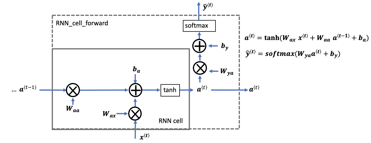
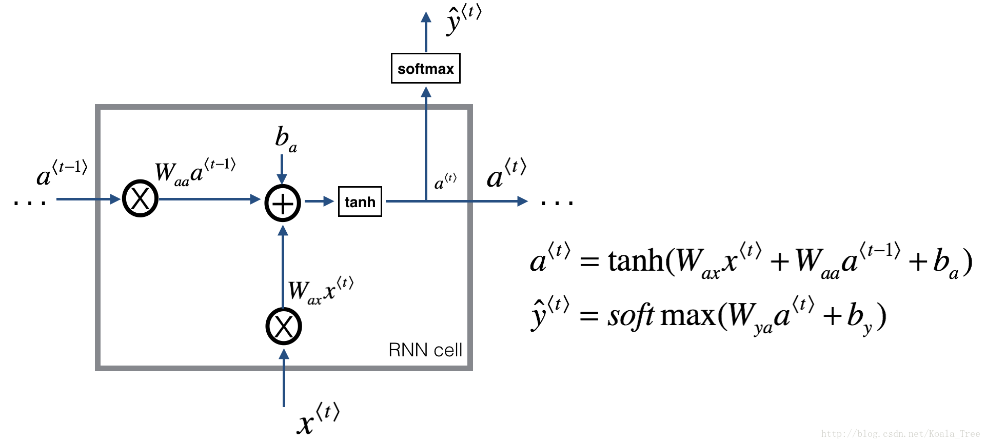
Figure 2: Basic RNN cell. Takes as input \(x^{\langle t \rangle}\) (current input) and \(a^{\langle t - 1\rangle}\) (previous hidden state containing information from the past), and outputs \(a^{\langle t \rangle}\) which is given to the next RNN cell and also used to predict \(y^{\langle t \rangle}\)
Instructions:
-
Compute the hidden state with tanh activation: \(a^{\langle t \rangle} = \tanh(W_{aa} a^{\langle t-1 \rangle} + W_{ax} x^{\langle t \rangle} + b_a)\).
-
Using your new hidden state \(a^{\langle t \rangle}\), compute the prediction \(\hat{y}^{\langle t \rangle} = softmax(W_{ya} a^{\langle t \rangle} + b_y)\). We provided you a function:
softmax. -
Store \((a^{\langle t \rangle}, a^{\langle t-1 \rangle}, x^{\langle t \rangle}, parameters)\) in cache
-
Return \(a^{\langle t \rangle}\) , \(y^{\langle t \rangle}\) and cache
We will vectorize over \(m\) examples. Thus, \(x^{\langle t \rangle}\) will have dimension \((n_x,m)\), and \(a^{\langle t \rangle}\) will have dimension \((n_a,m)\).
# GRADED FUNCTION: rnn_cell_forward

def rnn_cell_forward(xt, a_prev, parameters):
    """
    Implements a single forward step of the RNN-cell as described in Figure (2)

    Arguments:
    xt -- your input data at timestep "t", numpy array of shape (n_x, m).
    a_prev -- Hidden state at timestep "t-1", numpy array of shape (n_a, m)
    parameters -- python dictionary containing:
                        Wax -- Weight matrix multiplying the input, numpy array of shape (n_a, n_x)
                        Waa -- Weight matrix multiplying the hidden state, numpy array of shape (n_a, n_a)
                        Wya -- Weight matrix relating the hidden-state to the output, numpy array of shape (n_y, n_a)
                        ba --  Bias, numpy array of shape (n_a, 1)
                        by -- Bias relating the hidden-state to the output, numpy array of shape (n_y, 1)
    Returns:
    a_next -- next hidden state, of shape (n_a, m)
    yt_pred -- prediction at timestep "t", numpy array of shape (n_y, m)
    cache -- tuple of values needed for the backward pass, contains (a_next, a_prev, xt, parameters)
    """

    # Retrieve parameters from "parameters"
    Wax = parameters["Wax"]
    Waa = parameters["Waa"]
    Wya = parameters["Wya"]
    ba = parameters["ba"]
    by = parameters["by"]

    ### START CODE HERE ### (≈2 lines)
    # compute next activation state using the formula given above
    a_next = np.tanh(np.dot(Waa, a_prev) + np.dot(Wax, xt) + ba)
    # compute output of the current cell using the formula given above
    yt_pred = softmax(np.dot(Wya, a_next) + by)
    ### END CODE HERE ###

    # store values you need for backward propagation in cache
    cache = (a_next, a_prev, xt, parameters)

    return a_next, yt_pred, cache
测试:
np.random.seed(1)
xt = np.random.randn(3,10)
a_prev = np.random.randn(5,10)
Waa = np.random.randn(5,5)
Wax = np.random.randn(5,3)
Wya = np.random.randn(2,5)
ba = np.random.randn(5,1)
by = np.random.randn(2,1)
parameters = {"Waa": Waa, "Wax": Wax, "Wya": Wya, "ba": ba, "by": by}

a_next, yt_pred, cache = rnn_cell_forward(xt, a_prev, parameters)
print("a_next[4] = ", a_next[4])
print("a_next.shape = ", a_next.shape)
print("yt_pred[1] =", yt_pred[1])
print("yt_pred.shape = ", yt_pred.shape)
a_next[4] = [ 0.59584544 0.18141802 0.61311866 0.99808218 0.85016201 0.99980978
-0.18887155 0.99815551 0.6531151 0.82872037]
a_next.shape = (5, 10)
yt_pred[1] = [0.9888161 0.01682021 0.21140899 0.36817467 0.98988387 0.88945212
0.36920224 0.9966312 0.9982559 0.17746526]
yt_pred.shape = (2, 10)
1.2 RNN的前向传播
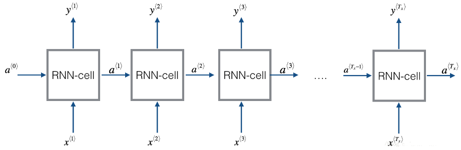
一个RNN是刚刚构建的 cell 的重复, 如果输入的数据序列经过10个时间步,那么将复制RNN单元10次,每个单元将前一个单元中的hidden state(\(a^{\langle t-1 \rangle}\)) 和当前时间步的输入数据(\(x^{\langle t \rangle}\)) 作为输入。它输出当前 time-step的 a hidden state (\(a^{\langle t \rangle}\)) and a prediction (\(y^{\langle t \rangle}\)).

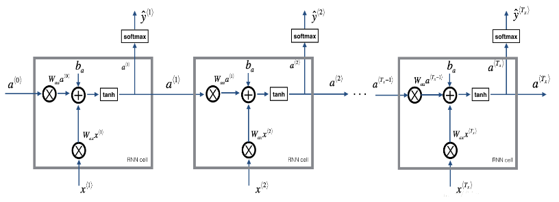
Figure 3: Basic RNN. The input sequence \(x = (x^{\langle 1 \rangle}, x^{\langle 2 \rangle}, ..., x^{\langle T_x \rangle})\) is carried over \(T_x\) time steps. The network outputs \(y = (y^{\langle 1 \rangle}, y^{\langle 2 \rangle}, ..., y^{\langle T_x \rangle})\).
Instructions:
-
创建 维度\((n_{a}, m, T_{x})\) 的零向量zeros (\(a\)) 将保存 由RNN计算的 所有 the hidden states
a. -
使用 \(a_0\) (initial hidden state) 初始化 the "next" hidden state .
-
开始循环所有的 time-step, your incremental index is \(t\) :
-
使用
rnn_cell_forward函数 更新 "next" hidden state and the cache. -
使用 \(a\) 来保存 "next" hidden state (\(t^{th}\) position).
-
使用 \(y\) 来保存预测值(prediction).
-
把
cache保存到caches列表中.
-
-
返回 \(a\), \(y\) and caches
Hints:
- Create a 3D array of zeros, \(a\) of shape \((n_{a}, m, T_{x})\) that will store all the hidden states computed by the RNN.
- Create a 3D array of zeros, \(\hat{y}\), of shape \((n_{y}, m, T_{x})\) that will store the predictions.
- Note that in this case, \(T_{y} = T_{x}\) (the prediction and input have the same number of time steps).
- Initialize the 2D hidden state
a_nextby setting it equal to the initial hidden state, \(a_{0}\). - At each time step \(t\):
- Get \(x^{\langle t \rangle}\), which is a 2D slice of \(x\) for a single time step \(t\).
- \(x^{\langle t \rangle}\) has shape \((n_{x}, m)\)
- \(x\) has shape \((n_{x}, m, T_{x})\)
- Update the 2D hidden state \(a^{\langle t \rangle}\) (variable name
a_next), the prediction \(\hat{y}^{\langle t \rangle}\) and the cache by runningrnn_cell_forward.- \(a^{\langle t \rangle}\) has shape \((n_{a}, m)\)
- Store the 2D hidden state in the 3D tensor \(a\), at the \(t^{th}\) position.
- \(a\) has shape \((n_{a}, m, T_{x})\)
- Store the 2D \(\hat{y}^{\langle t \rangle}\) prediction (variable name
yt_pred) in the 3D tensor \(\hat{y}_{pred}\) at the \(t^{th}\) position.- \(\hat{y}^{\langle t \rangle}\) has shape \((n_{y}, m)\)
- \(\hat{y}\) has shape \((n_{y}, m, T_x)\)
- Append the cache to the list of caches.
- Get \(x^{\langle t \rangle}\), which is a 2D slice of \(x\) for a single time step \(t\).
- Return the 3D tensor \(a\) and \(\hat{y}\), as well as the list of caches.
# GRADED FUNCTION: rnn_forward

def rnn_forward(x, a0, parameters):
    """
    Implement the forward propagation of the recurrent neural network described in Figure (3).

    Arguments:
    x -- Input data for every time-step, of shape (n_x, m, T_x).
    a0 -- Initial hidden state, of shape (n_a, m)
    parameters -- python dictionary containing:
                        Waa -- Weight matrix multiplying the hidden state, numpy array of shape (n_a, n_a)
                        Wax -- Weight matrix multiplying the input, numpy array of shape (n_a, n_x)
                        Wya -- Weight matrix relating the hidden-state to the output, numpy array of shape (n_y, n_a)
                        ba --  Bias numpy array of shape (n_a, 1)
                        by -- Bias relating the hidden-state to the output, numpy array of shape (n_y, 1)

    Returns:
    a -- Hidden states for every time-step, numpy array of shape (n_a, m, T_x)
    y_pred -- Predictions for every time-step, numpy array of shape (n_y, m, T_x)
    caches -- tuple of values needed for the backward pass, contains (list of caches, x)
    """

    # Initialize "caches" which will contain the list of all caches
    caches = []

    # Retrieve dimensions from shapes of x and parameters["Wya"]
    n_x, m, T_x = x.shape
    n_y, n_a = parameters["Wya"].shape

    ### START CODE HERE ###

    # initialize "a" and "y" with zeros (≈2 lines)
    a = np.zeros((n_a, m, T_x))
    y_pred = np.zeros((n_y, m, T_x))

    # Initialize a_next (≈1 line)
    a_next = a0

    # loop over all time-steps
    for t in range(T_x):
        # Update next hidden state, compute the prediction, get the cache (≈1 line)
        a_next, yt_pred, cache = rnn_cell_forward(x[:,:,t], a_next, parameters)
        # Save the value of the new "next" hidden state in a (≈1 line)
        a[:,:,t] = a_next
        # Save the value of the prediction in y (≈1 line)
        y_pred[:,:,t] = yt_pred
        # Append "cache" to "caches" (≈1 line)
        caches.append(cache)

    ### END CODE HERE ###

    # store values needed for backward propagation in cache
    caches = (caches, x)

    return a, y_pred, caches
测试:
np.random.seed(1)
x = np.random.randn(3,10,4)
a0 = np.random.randn(5,10)
Waa = np.random.randn(5,5)
Wax = np.random.randn(5,3)
Wya = np.random.randn(2,5)
ba = np.random.randn(5,1)
by = np.random.randn(2,1)
parameters = {"Waa": Waa, "Wax": Wax, "Wya": Wya, "ba": ba, "by": by}

a, y_pred, caches = rnn_forward(x, a0, parameters)
print("a[4][1] = ", a[4][1])
print("a.shape = ", a.shape)
print("y_pred[1][3] =", y_pred[1][3])
print("y_pred.shape = ", y_pred.shape)
print("caches[1][1][3] =", caches[1][1][3])
print("len(caches) = ", len(caches))
a[4][1] = [-0.99999375 0.77911235 -0.99861469 -0.99833267]
a.shape = (5, 10, 4)
y_pred[1][3] = [0.79560373 0.86224861 0.11118257 0.81515947]
y_pred.shape = (2, 10, 4)
caches[1][1][3] = [-1.1425182 -0.34934272 -0.20889423 0.58662319]
len(caches) = 2
我们构建了循环神经网络的前向传播函数,这对于某些应用程序来说已经足够好了,但是它还存在梯度消失(vanishing gradient )的问题。当每个输出 \(y^{\langle t \rangle}\) 是根据 局部上下文("local" context) 来预测时,效果较好。(意思是输入 \(x^{\langle t' \rangle}\) ,其中 \(t'\) 与 \(t\) 相隔不太远).
接下来要构建一个更加复杂的 LSTM模型,它可以更好地解决梯度消失的问题,LSTM能够更好地记住一条信息,并且可以在很多time-steps中保存。
2. Long Short-Term Memory (LSTM) network
下图是LSTM模块:
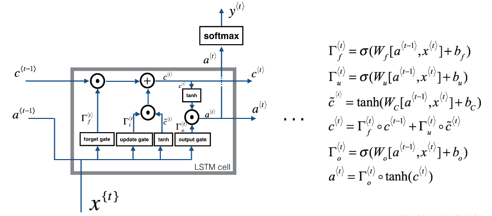
Figure 4: LSTM-cell. 它跟踪和更新每个time-step上的 单元状态(cell state) 或 记忆变量(memory variable) \(c^{\langle t \rangle}\), 这跟 \(a^{\langle t \rangle}\) 不同.
先来实现一个LSTM单元,只执行一个时间步,然后在循环中调用,以处理所有输入数据。
About the gates
- Forget gate
假设,我们正在阅读文本中的单词,并希望使用LSTM来跟踪语法结构,比如,主语是单数(singular)还是复数(plural)。如果主语从单数变为复数,我们需要找到一种方法来 摆脱 我们先前存储的单复数状态的记忆值。在LSTM中,遗忘门是这样做的:
其中, \(W_f\) 是控制遗忘门的权值,我们 concatenate \([a^{\langle t-1 \rangle}, x^{\langle t \rangle}]\) and multiply by \(W_f\),结果是得到了一个 vector \(\Gamma_f^{\langle t \rangle}\),其值在0 与 1 之间。这个 forget gate vector 将与 前一个单元状态(cell state) \(c^{\langle t-1 \rangle}\) 元素相乘。
因此,如果 \(\Gamma_f^{\langle t \rangle}\) 的一个值是 0 (或 \(\approx\) 0) ,则意味着 LSTM 应该删除这条信息 ( the singular subject) 在相应的\(c^{\langle t-1 \rangle}\)组成部分中。如果其中有值为 1,那么 LSTM 将保留信息。
- Update gate
一旦我们忘记过去所讨论的主语是单数,我们需要找到一种方法来更新它,以反映新的主语现在是复数。这里是更新门(update gate)的公式
与遗忘门相似,\(\Gamma_u^{\langle t \rangle}\) 向量的值在0与 1之间。为了计算 \(c^{\langle t \rangle}\),它会与 \(\tilde{c}^{\langle t \rangle}\) 元素相乘。
- Updating the cell
为了更新主语,我们需要创建一个新的向量,我们可以将其添加到之前的单元状态中(cell state)。公式为:
最后,新的单元状态(cell state)是:
- Output gate
为了决定我们将使用哪种输出,使用下列公式:
2.1 LSTM cell
Instructions:
-
把 \(a^{\langle t-1 \rangle}\) 和 \(x^{\langle t \rangle}\) 连接起来变成一个矩阵: \(concat = \begin{bmatrix} a^{\langle t-1 \rangle} \\ x^{\langle t \rangle} \end{bmatrix}\).
-
计算公式 1-6,你可以使用
sigmoid()(provided) 和np.tanh(). -
计算 prediction \(y^{\langle t \rangle}\). 你可以使用
softmax()(provided).
# GRADED FUNCTION: lstm_cell_forward

def lstm_cell_forward(xt, a_prev, c_prev, parameters):
    """
    Implement a single forward step of the LSTM-cell as described in Figure (4)

    Arguments:
    xt -- your input data at timestep "t", numpy array of shape (n_x, m).
    a_prev -- Hidden state at timestep "t-1", numpy array of shape (n_a, m)
    c_prev -- Memory state at timestep "t-1", numpy array of shape (n_a, m)
    parameters -- python dictionary containing:
                        Wf -- Weight matrix of the forget gate, numpy array of shape (n_a, n_a + n_x)
                        bf -- Bias of the forget gate, numpy array of shape (n_a, 1)
                        Wi -- Weight matrix of the update gate, numpy array of shape (n_a, n_a + n_x)
                        bi -- Bias of the update gate, numpy array of shape (n_a, 1)
                        Wc -- Weight matrix of the first "tanh", numpy array of shape (n_a, n_a + n_x)
                        bc --  Bias of the first "tanh", numpy array of shape (n_a, 1)
                        Wo -- Weight matrix of the output gate, numpy array of shape (n_a, n_a + n_x)
                        bo --  Bias of the output gate, numpy array of shape (n_a, 1)
                        Wy -- Weight matrix relating the hidden-state to the output, numpy array of shape (n_y, n_a)
                        by -- Bias relating the hidden-state to the output, numpy array of shape (n_y, 1)

    Returns:
    a_next -- next hidden state, of shape (n_a, m)
    c_next -- next memory state, of shape (n_a, m)
    yt_pred -- prediction at timestep "t", numpy array of shape (n_y, m)
    cache -- tuple of values needed for the backward pass, contains (a_next, c_next, a_prev, c_prev, xt, parameters)

    Note: ft/it/ot stand for the forget/update/output gates, cct stands for the candidate value (c tilde),
          c stands for the memory value
    """

    # Retrieve parameters from "parameters"
    Wf = parameters["Wf"]
    bf = parameters["bf"]
    Wi = parameters["Wi"]
    bi = parameters["bi"]
    Wc = parameters["Wc"]
    bc = parameters["bc"]
    Wo = parameters["Wo"]
    bo = parameters["bo"]
    Wy = parameters["Wy"]
    by = parameters["by"]

    # Retrieve dimensions from shapes of xt and Wy
    n_x, m = xt.shape
    n_y, n_a = Wy.shape

    ### START CODE HERE ###
    # Concatenate a_prev and xt (≈3 lines)
    concat = np.zeros((n_a+n_x, m))
    concat[: n_a, :] = a_prev
    concat[n_a :, :] = xt

    # Compute values for ft, it, cct, c_next, ot, a_next using the formulas given figure (4) (≈6 lines)
    ft = sigmoid(np.dot(Wf, concat) + bf)
    it = sigmoid(np.dot(Wi, concat) + bi)
    cct = np.tanh(np.dot(Wc, concat) + bc)
    c_next = ft * c_prev + it * cct
    ot = sigmoid(np.dot(Wo, concat) + bo)
    a_next = ot * np.tanh(c_next)

    c_next = ft * c_prev + it * cct
    ot = sigmoid(np.dot(Wo,concat)+bo)
    a_next = ot * np.tanh(c_next)

    # Compute prediction of the LSTM cell (≈1 line)
    yt_pred = softmax(np.dot(Wy, a_next) + by)
    ### END CODE HERE ###

    # store values needed for backward propagation in cache
    cache = (a_next, c_next, a_prev, c_prev, ft, it, cct, ot, xt, parameters)

    return a_next, c_next, yt_pred, cache
测试
np.random.seed(1)
xt = np.random.randn(3,10)
a_prev = np.random.randn(5,10)
c_prev = np.random.randn(5,10)
Wf = np.random.randn(5, 5+3)
bf = np.random.randn(5,1)
Wi = np.random.randn(5, 5+3)
bi = np.random.randn(5,1)
Wo = np.random.randn(5, 5+3)
bo = np.random.randn(5,1)
Wc = np.random.randn(5, 5+3)
bc = np.random.randn(5,1)
Wy = np.random.randn(2,5)
by = np.random.randn(2,1)

parameters = {"Wf": Wf, "Wi": Wi, "Wo": Wo, "Wc": Wc, "Wy": Wy, "bf": bf, "bi": bi, "bo": bo, "bc": bc, "by": by}

a_next, c_next, yt, cache = lstm_cell_forward(xt, a_prev, c_prev, parameters)
print("a_next[4] = ", a_next[4])
print("a_next.shape = ", c_next.shape)
print("c_next[2] = ", c_next[2])
print("c_next.shape = ", c_next.shape)
print("yt[1] =", yt[1])
print("yt.shape = ", yt.shape)
print("cache[1][3] =", cache[1][3])
print("len(cache) = ", len(cache))
a_next[4] = [-0.66408471 0.0036921 0.02088357 0.22834167 -0.85575339 0.00138482
0.76566531 0.34631421 -0.00215674 0.43827275]
a_next.shape = (5, 10)
c_next[2] = [ 0.63267805 1.00570849 0.35504474 0.20690913 -1.64566718 0.11832942
0.76449811 -0.0981561 -0.74348425 -0.26810932]
c_next.shape = (5, 10)
yt[1] = [0.79913913 0.15986619 0.22412122 0.15606108 0.97057211 0.31146381
0.00943007 0.12666353 0.39380172 0.07828381]
yt.shape = (2, 10)
cache[1][3] = [-0.16263996 1.03729328 0.72938082 -0.54101719 0.02752074 -0.30821874
0.07651101 -1.03752894 1.41219977 -0.37647422]
len(cache) = 10
2.2 Forward pass for LSTM
我们已经实现了LSTM单元的一个时间步的前向传播,现在我们要对LSTM网络进行前向传播进行计算
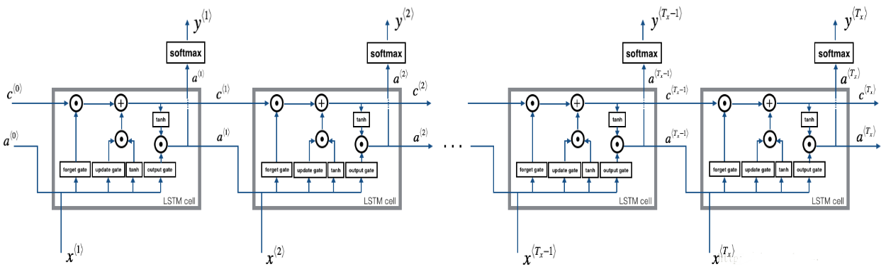
Figure 4: LSTM over multiple time-steps.
Exercise: Implement lstm_forward() to run an LSTM over \(T_x\) time-steps.
Note: \(c^{\langle 0 \rangle}\) is initialized with zeros.
# GRADED FUNCTION: lstm_forward

def lstm_forward(x, a0, parameters):
    """
    Implement the forward propagation of the recurrent neural network using an LSTM-cell described in Figure (3).

    Arguments:
    x -- Input data for every time-step, of shape (n_x, m, T_x).
    a0 -- Initial hidden state, of shape (n_a, m)
    parameters -- python dictionary containing:
                        Wf -- Weight matrix of the forget gate, numpy array of shape (n_a, n_a + n_x)
                        bf -- Bias of the forget gate, numpy array of shape (n_a, 1)
                        Wi -- Weight matrix of the update gate, numpy array of shape (n_a, n_a + n_x)
                        bi -- Bias of the update gate, numpy array of shape (n_a, 1)
                        Wc -- Weight matrix of the first "tanh", numpy array of shape (n_a, n_a + n_x)
                        bc -- Bias of the first "tanh", numpy array of shape (n_a, 1)
                        Wo -- Weight matrix of the output gate, numpy array of shape (n_a, n_a + n_x)
                        bo -- Bias of the output gate, numpy array of shape (n_a, 1)
                        Wy -- Weight matrix relating the hidden-state to the output, numpy array of shape (n_y, n_a)
                        by -- Bias relating the hidden-state to the output, numpy array of shape (n_y, 1)

    Returns:
    a -- Hidden states for every time-step, numpy array of shape (n_a, m, T_x)
    y -- Predictions for every time-step, numpy array of shape (n_y, m, T_x)
    caches -- tuple of values needed for the backward pass, contains (list of all the caches, x)
    """

    # Initialize "caches", which will track the list of all the caches
    caches = []

    ### START CODE HERE ###
    # Retrieve dimensions from shapes of x and parameters['Wy'] (≈2 lines)
    n_x, m, T_x = x.shape
    n_y, n_a = parameters['Wy'].shape

    # initialize "a", "c" and "y" with zeros (≈3 lines)
    a = np.zeros((n_a, m, T_x))
    c = np.zeros((n_a, m, T_x))
    y = np.zeros((n_y, m, T_x))

    # Initialize a_next and c_next (≈2 lines)
    a_next = a0
    c_next = np.zeros((n_a, 1))

    # loop over all time-steps
    for t in range(T_x):
        # Update next hidden state, next memory state, compute the prediction, get the cache (≈1 line)
        # a_next, c_next, yt_pred, cache
        a_next, c_next, yt, cache = lstm_cell_forward(x[:,:,t], a_next, c_next, parameters)
        # Save the value of the new "next" hidden state in a (≈1 line)
        a[:,:,t] = a_next
        # Save the value of the prediction in y (≈1 line)
        y[:,:,t] = yt
        # Save the value of the next cell state (≈1 line)
        c[:,:,t] = c_next
        # Append the cache into caches (≈1 line)
        caches.append(cache)

    ### END CODE HERE ###

    # store values needed for backward propagation in cache
    caches = (caches, x)

    return a, y, c, caches
测试:
np.random.seed(1)
x = np.random.randn(3,10,7)
a0 = np.random.randn(5,10)
Wf = np.random.randn(5, 5+3)
bf = np.random.randn(5,1)
Wi = np.random.randn(5, 5+3)
bi = np.random.randn(5,1)
Wo = np.random.randn(5, 5+3)
bo = np.random.randn(5,1)
Wc = np.random.randn(5, 5+3)
bc = np.random.randn(5,1)
Wy = np.random.randn(2,5)
by = np.random.randn(2,1)

parameters = {"Wf": Wf, "Wi": Wi, "Wo": Wo, "Wc": Wc, "Wy": Wy, "bf": bf, "bi": bi, "bo": bo, "bc": bc, "by": by}

a, y, c, caches = lstm_forward(x, a0, parameters)
print("a[4][3][6] = ", a[4][3][6])
print("a.shape = ", a.shape)
print("y[1][4][3] =", y[1][4][3])
print("y.shape = ", y.shape)
print("caches[1][1[1]] =", caches[1][1][1])
print("c[1][2][1]", c[1][2][1])
print("len(caches) = ", len(caches))
a[4][3][6] = 0.17211776753291672
a.shape = (5, 10, 7)
y[1][4][3] = 0.9508734618501101
y.shape = (2, 10, 7)
caches[1][1[1]] = [ 0.82797464 0.23009474 0.76201118 -0.22232814 -0.20075807 0.18656139
0.41005165]
c[1][2][1] -0.8555449167181981
len(caches) = 2
3. Backpropagation in recurrent neural networks
在循环神经网络中,我们可以计算与成本相关的导数,以便更新参数。
3.1 基本的RNN网络的反向传播
We will start by computing the backward pass for the basic RNN-cell.
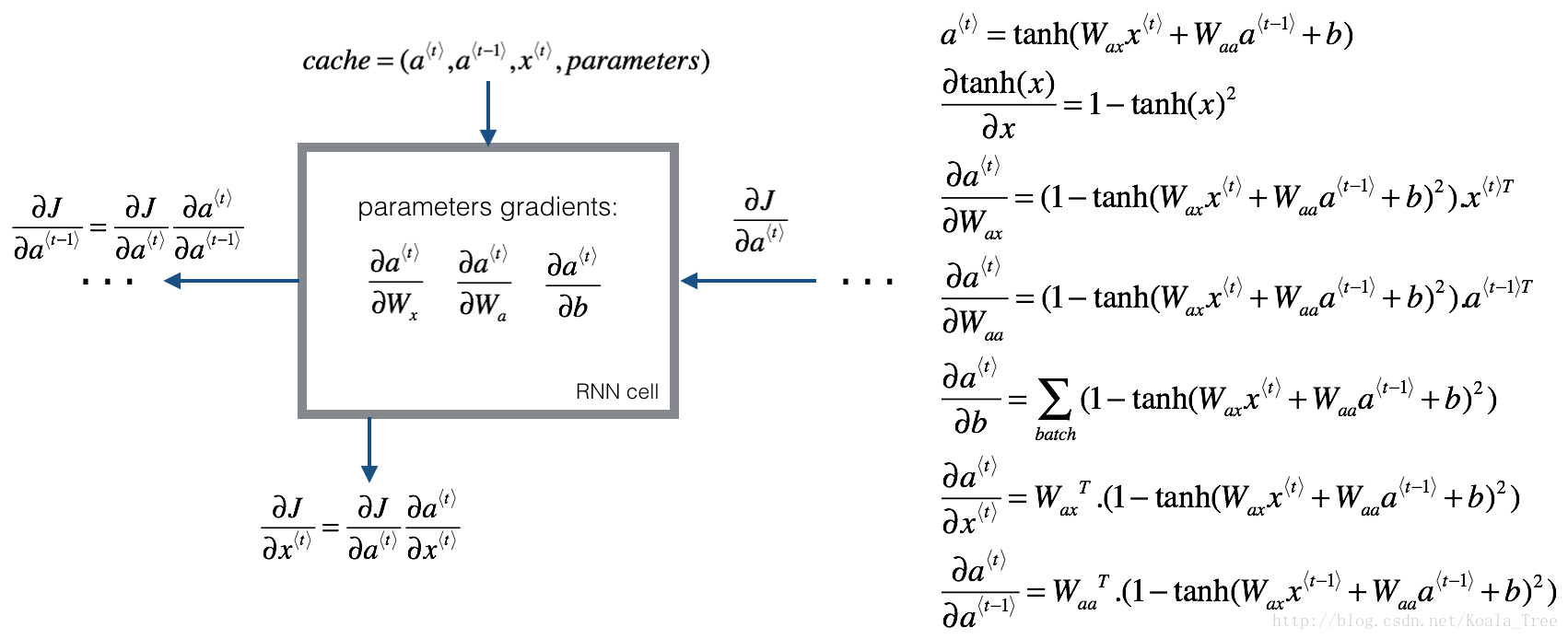
Figure 5: RNN-cell's backward pass. 就像在fully-connected neural network, the cost function \(J\) 的导数通过遵循链式法则从RNN进行反向传播。 链式法则也用于计算 \((\frac{\partial J}{\partial W_{ax}},\frac{\partial J}{\partial W_{aa}},\frac{\partial J}{\partial b})\) 来更新 parameters \((W_{ax}, W_{aa}, b_a)\).
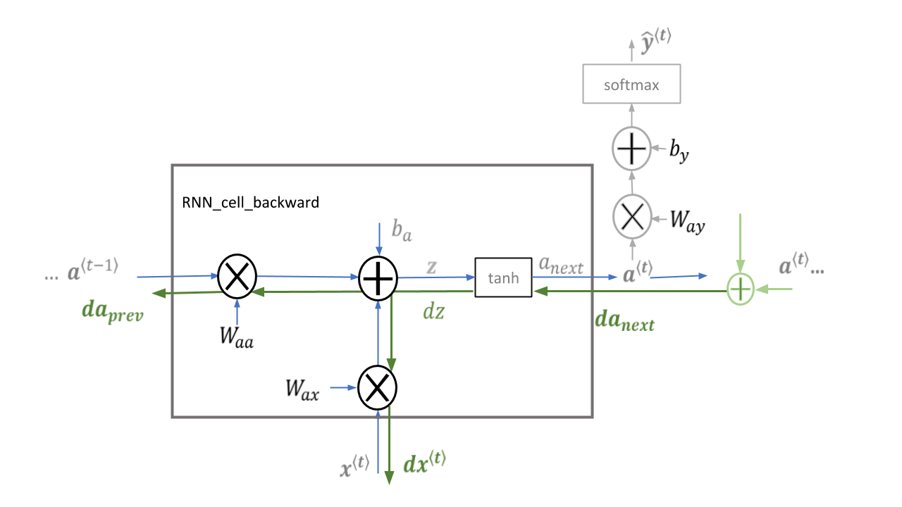
Figure 7: This implementation of rnn_cell_backward does not include the output dense layer and softmax which are included in rnn_cell_forward.
\(da_{next}\) is \(\frac{\partial{J}}{\partial a^{\langle t \rangle}}\) and includes loss from previous stages and current stage output logic. The addition shown in green will be part of your implementation of rnn_backward.
Deriving the one step backward functions:
单步反向传播的推导:为了计算rnn_cell_backward,我们需要计算下面的公式:
\(\tanh\) 的导数是 \(1-\tanh(x)^2\). 证明. 注意: \(\text{sech}(x)^2 = 1 - \tanh(x)^2\)
相似于,对于 \(\frac{ \partial a^{\langle t \rangle} } {\partial W_{ax}}, \frac{ \partial a^{\langle t \rangle} } {\partial W_{aa}}, \frac{ \partial a^{\langle t \rangle} } {\partial b}\), \(\tanh(u)\) 的导数是 \((1-\tanh(u)^2)du\).
dtanh = da_next * (1 - np.square(np.tanh(np.dot(Wax, xt) + np.dot(Waa, a_prev) + ba)))
Equations
To compute the rnn_cell_backward you can utilize the following equations. It is a good exercise to derive them by hand. Here, \(*\) denotes element-wise multiplication while the absence of a symbol indicates matrix multiplication.
def rnn_cell_backward(da_next, cache):
    """
    Implements the backward pass for the RNN-cell (single time-step).

    Arguments:
    da_next -- Gradient of loss with respect to next hidden state
    cache -- python dictionary containing useful values (output of rnn_cell_forward())

    Returns:
    gradients -- python dictionary containing:
                        dx -- Gradients of input data, of shape (n_x, m)
                        da_prev -- Gradients of previous hidden state, of shape (n_a, m)
                        dWax -- Gradients of input-to-hidden weights, of shape (n_a, n_x)
                        dWaa -- Gradients of hidden-to-hidden weights, of shape (n_a, n_a)
                        dba -- Gradients of bias vector, of shape (n_a, 1)
    """

    # Retrieve values from cache
    (a_next, a_prev, xt, parameters) = cache

    # Retrieve values from parameters
    Wax = parameters["Wax"]
    Waa = parameters["Waa"]
    Wya = parameters["Wya"]
    ba = parameters["ba"]
    by = parameters["by"]

    ### START CODE HERE ###
    # compute the gradient of tanh with respect to a_next (≈1 line)
    dtanh = da_next * (1 - np.square(np.tanh(np.dot(Wax, xt) + np.dot(Waa, a_prev) + ba)))

    # compute the gradient of the loss with respect to Wax (≈2 lines)
    dxt = np.dot(Wax.T, dtanh)
    dWax = np.dot(dtanh, xt.T)

    # compute the gradient with respect to Waa (≈2 lines)
    da_prev = np.dot(Waa.T, dtanh)
    dWaa = np.dot(dtanh, a_prev.T)

    # compute the gradient with respect to b (≈1 line)
    dba = np.sum(dtanh, axis = 1, keepdims = True)

    ### END CODE HERE ###

    # Store the gradients in a python dictionary
    gradients = {"dxt": dxt, "da_prev": da_prev, "dWax": dWax, "dWaa": dWaa, "dba": dba}

    return gradients
测试:
np.random.seed(1)
xt = np.random.randn(3,10)
a_prev = np.random.randn(5,10)
Wax = np.random.randn(5,3)
Waa = np.random.randn(5,5)
Wya = np.random.randn(2,5)
b = np.random.randn(5,1)
by = np.random.randn(2,1)
parameters = {"Wax": Wax, "Waa": Waa, "Wya": Wya, "ba": ba, "by": by}

a_next, yt, cache = rnn_cell_forward(xt, a_prev, parameters)

da_next = np.random.randn(5,10)
gradients = rnn_cell_backward(da_next, cache)
print("gradients[\"dxt\"][1][2] =", gradients["dxt"][1][2])
print("gradients[\"dxt\"].shape =", gradients["dxt"].shape)
print("gradients[\"da_prev\"][2][3] =", gradients["da_prev"][2][3])
print("gradients[\"da_prev\"].shape =", gradients["da_prev"].shape)
print("gradients[\"dWax\"][3][1] =", gradients["dWax"][3][1])
print("gradients[\"dWax\"].shape =", gradients["dWax"].shape)
print("gradients[\"dWaa\"][1][2] =", gradients["dWaa"][1][2])
print("gradients[\"dWaa\"].shape =", gradients["dWaa"].shape)
print("gradients[\"dba\"][4] =", gradients["dba"][4])
print("gradients[\"dba\"].shape =", gradients["dba"].shape)
gradients["dxt"][1][2] = -0.4605641030588796
gradients["dxt"].shape = (3, 10)
gradients["da_prev"][2][3] = 0.08429686538067718
gradients["da_prev"].shape = (5, 10)
gradients["dWax"][3][1] = 0.3930818739219304
gradients["dWax"].shape = (5, 3)
gradients["dWaa"][1][2] = -0.2848395578696067
gradients["dWaa"].shape = (5, 5)
gradients["dba"][4] = [0.80517166]
gradients["dba"].shape = (5, 1)
Backward pass through the RNN
计算 每个time-step关于 \(a^{\langle t \rangle}\) 代价的梯度 是有用的,因为它帮助梯度 向前一个 RNN-cell 反向传播。从结尾开始,迭代所有time steps,每一步,实现 \(db_a\), \(dW_{aa}\), \(dW_{ax}\), 并且存储 \(dx\).
Instructions:
实现 rnn_backward函数. 首先,初始化 回归变量为0,然后,循环每个time-steps,通过调用 rnn_cell_backward,更新其他变量.
def rnn_backward(da, caches):
    """
    Implement the backward pass for a RNN over an entire sequence of input data.

    Arguments:
    da -- Upstream gradients of all hidden states, of shape (n_a, m, T_x)
    caches -- tuple containing information from the forward pass (rnn_forward)

    Returns:
    gradients -- python dictionary containing:
                        dx -- Gradient w.r.t. the input data, numpy-array of shape (n_x, m, T_x)
                        da0 -- Gradient w.r.t the initial hidden state, numpy-array of shape (n_a, m)
                        dWax -- Gradient w.r.t the input's weight matrix, numpy-array of shape (n_a, n_x)
                        dWaa -- Gradient w.r.t the hidden state's weight matrix, numpy-arrayof shape (n_a, n_a)
                        dba -- Gradient w.r.t the bias, of shape (n_a, 1)
    """

    ### START CODE HERE ###

    # Retrieve values from the first cache (t=1) of caches (≈2 lines)
    (caches, x) = caches

    (a1, a0, x1, parameters) = caches[0]

    # Retrieve dimensions from da's and x1's shapes (≈2 lines)
    n_a, m, T_x = da.shape
    n_x, m = x1.shape

    # initialize the gradients with the right sizes (≈6 lines)
    dx = np.zeros((n_x, m, T_x))
    dWax = np.zeros((n_a, n_x))
    dWaa = np.zeros((n_a, n_a))
    dba = np.zeros((n_a, 1))
    da0 = np.zeros((n_a, m))
    da_prevt = np.zeros((n_a, 1))

    # Loop through all the time steps
    for t in reversed(range(T_x)):
        # Compute gradients at time step t. Choose wisely the "da_next" and the "cache" to use in the backward propagation step. (≈1 line)
        gradients = rnn_cell_backward(da[:,:,t] + da_prevt, caches[t])
        # Retrieve derivatives from gradients (≈ 1 line)
        dxt, da_prevt, dWaxt, dWaat, dbat = gradients['dxt'], gradients['da_prev'], gradients['dWax'], gradients['dWaa'], gradients['dba']
        # Increment global derivatives w.r.t parameters by adding their derivative at time-step t (≈4 lines)
        dx[:, :, t] = dxt
        dWax += dWaxt
        dWaa += dWaat
        dba += dbat

    # Set da0 to the gradient of a which has been backpropagated through all time-steps (≈1 line)
    da0 = da_prevt
    ### END CODE HERE ###

    # Store the gradients in a python dictionary
    gradients = {"dx": dx, "da0": da0, "dWax": dWax, "dWaa": dWaa,"dba": dba}

    return gradients
测试:
np.random.seed(1)
x = np.random.randn(3,10,4)
a0 = np.random.randn(5,10)
Wax = np.random.randn(5,3)
Waa = np.random.randn(5,5)
Wya = np.random.randn(2,5)
ba = np.random.randn(5,1)
by = np.random.randn(2,1)
parameters = {"Wax": Wax, "Waa": Waa, "Wya": Wya, "ba": ba, "by": by}
a, y, caches = rnn_forward(x, a0, parameters)
da = np.random.randn(5, 10, 4)
gradients = rnn_backward(da, caches)

print("gradients[\"dx\"][1][2] =", gradients["dx"][1][2])
print("gradients[\"dx\"].shape =", gradients["dx"].shape)
print("gradients[\"da0\"][2][3] =", gradients["da0"][2][3])
print("gradients[\"da0\"].shape =", gradients["da0"].shape)
print("gradients[\"dWax\"][3][1] =", gradients["dWax"][3][1])
print("gradients[\"dWax\"].shape =", gradients["dWax"].shape)
print("gradients[\"dWaa\"][1][2] =", gradients["dWaa"][1][2])
print("gradients[\"dWaa\"].shape =", gradients["dWaa"].shape)
print("gradients[\"dba\"][4] =", gradients["dba"][4])
print("gradients[\"dba\"].shape =", gradients["dba"].shape)
gradients["dx"][1][2] = [-2.07101689 -0.59255627 0.02466855 0.01483317]
gradients["dx"].shape = (3, 10, 4)
gradients["da0"][2][3] = -0.31494237512664996
gradients["da0"].shape = (5, 10)
gradients["dWax"][3][1] = 11.264104496527777
gradients["dWax"].shape = (5, 3)
gradients["dWaa"][1][2] = 2.3033331265798935
gradients["dWaa"].shape = (5, 5)
gradients["dba"][4] = [-0.74747722]
gradients["dba"].shape = (5, 1)
3.2 LSTM backward pass
3.21 One step backward
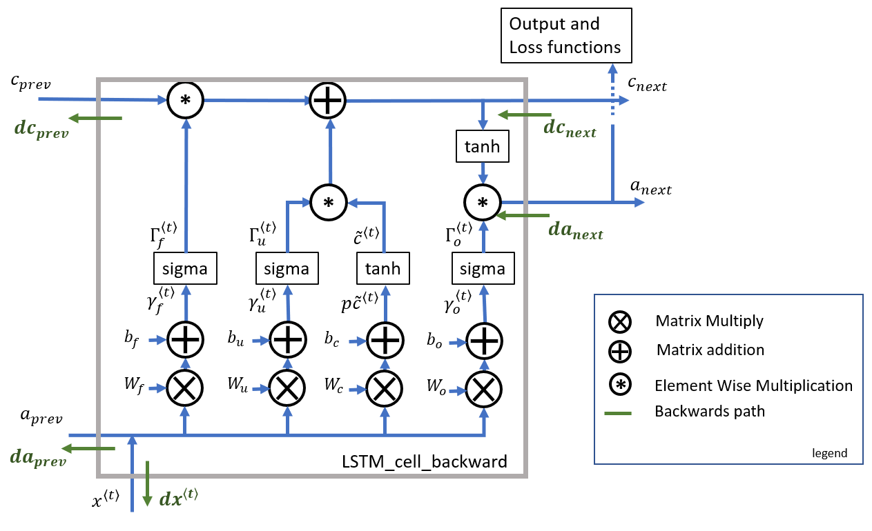
3.22 gate derivatives
3.23 parameter derivatives
\(dW_f = d\Gamma_f^{\langle t \rangle} \begin{bmatrix} a_{prev} \\ x_t\end{bmatrix}^T \tag{11}\)
\(dW_u = d\Gamma_u^{\langle t \rangle} \begin{bmatrix} a_{prev} \\ x_t\end{bmatrix}^T \tag{12}\)
\(dW_c = dp\widetilde c^{\langle t \rangle} \begin{bmatrix} a_{prev} \\ x_t\end{bmatrix}^T \tag{13}\)
\(dW_o = d\Gamma_o^{\langle t \rangle} \begin{bmatrix} a_{prev} \\ x_t\end{bmatrix}^T \tag{14}\)
为了计算 \(db_f, db_u, db_c, db_o\) 你需要在 \(d\Gamma_f^{\langle t \rangle}, d\Gamma_u^{\langle t \rangle}, dp\tilde c^{\langle t \rangle}, d\Gamma_o^{\langle t \rangle}\) 上在horizontal axis(axis=1) 进行求和。需要使用 keep_dims = True 选项.
\(\displaystyle db_f = \sum_{batch}d\Gamma_f^{\langle t \rangle}\tag{15}\)
\(\displaystyle db_u = \sum_{batch}d\Gamma_u^{\langle t \rangle}\tag{16}\)
\(\displaystyle db_c = \sum_{batch}d\Gamma_c^{\langle t \rangle}\tag{17}\)
\(\displaystyle db_o = \sum_{batch}d\Gamma_o^{\langle t \rangle}\tag{18}\)
最后,需要计算先前隐藏状态(the previous hidden state), 先前记忆单元(previous memory state), 和 输入(input) 的导数
这里,方程19的权重是第一个n_a,(比如: \(W_f = W_f[:,:n_a]\) 等)
方程21的权重从n_a到结尾,(比如: \(W_f = W_f[:,n_a:]\) 等)
Exercise: Implement lstm_cell_backward 通过实现公式 \(7-18\).
def lstm_cell_backward(da_next, dc_next, cache):
    """
    Implement the backward pass for the LSTM-cell (single time-step).

    Arguments:
    da_next -- Gradients of next hidden state, of shape (n_a, m)
    dc_next -- Gradients of next cell state, of shape (n_a, m)
    cache -- cache storing information from the forward pass

    Returns:
    gradients -- python dictionary containing:
                        dxt -- Gradient of input data at time-step t, of shape (n_x, m)
                        da_prev -- Gradient w.r.t. the previous hidden state, numpy array of shape (n_a, m)
                        dc_prev -- Gradient w.r.t. the previous memory state, of shape (n_a, m, T_x)
                        dWf -- Gradient w.r.t. the weight matrix of the forget gate, numpy array of shape (n_a, n_a + n_x)
                        dWi -- Gradient w.r.t. the weight matrix of the update gate, numpy array of shape (n_a, n_a + n_x)
                        dWc -- Gradient w.r.t. the weight matrix of the memory gate, numpy array of shape (n_a, n_a + n_x)
                        dWo -- Gradient w.r.t. the weight matrix of the output gate, numpy array of shape (n_a, n_a + n_x)
                        dbf -- Gradient w.r.t. biases of the forget gate, of shape (n_a, 1)
                        dbi -- Gradient w.r.t. biases of the update gate, of shape (n_a, 1)
                        dbc -- Gradient w.r.t. biases of the memory gate, of shape (n_a, 1)
                        dbo -- Gradient w.r.t. biases of the output gate, of shape (n_a, 1)
    """

    # Retrieve information from "cache"
    (a_next, c_next, a_prev, c_prev, ft, it, cct, ot, xt, parameters) = cache

    ### START CODE HERE ###
    # Retrieve dimensions from xt's and a_next's shape (≈2 lines)
    n_x, m = xt.shape
    n_a, m = a_next.shape

    # Compute gates related derivatives, you can find their values can be found by looking carefully at equations (7) to (10) (≈4 lines)
    dot = da_next * np.tanh(c_next) * ot * (1-ot)
    dcct = (dc_next * it + ot * (1 - np.square(np.tanh(c_next))) * it * da_next) * (1 - np.square(cct))
    dit = (dc_next * cct + ot * (1 - np.square(np.tanh(c_next))) * cct * da_next) * it * (1 - it)
    dft = (dc_next * c_prev + ot * (1 - np.square(np.tanh(c_next))) * c_prev * da_next) * ft * (1 - ft)

    # Compute parameters related derivatives. Use equations (11)-(14) (≈8 lines)
    concat = np.concatenate((a_prev, xt), axis=0).T
    dWf = np.dot(dft, concat)
    dWi = np.dot(dit, concat)
    dWc = np.dot(dcct, concat)
    dWo = np.dot(dot, concat)
    dbf = np.sum(dft, axis=1, keepdims=True)
    dbi = np.sum(dit, axis=1, keepdims=True)
    dbc = np.sum(dcct, axis=1, keepdims=True)
    dbo = np.sum(dot, axis=1, keepdims=True)

    # Compute derivatives w.r.t previous hidden state, previous memory state and input. Use equations (15)-(17). (≈3 lines)
    da_prev = np.dot(parameters['Wf'][:,:n_a].T, dft) +  np.dot(parameters["Wi"][:, :n_a].T, dit) + np.dot(parameters['Wc'][:,:n_a].T, dcct) + np.dot(parameters['Wo'][:,:n_a].T, dot)
    dc_prev = dc_next * ft + ot * (1-np.square(np.tanh(c_next))) * ft * da_next
    dxt = np.dot(parameters['Wf'][:, n_a:].T, dft) + np.dot(parameters["Wi"][:, n_a:].T, dit)+ np.dot(parameters['Wc'][:,n_a:].T,dcct) + np.dot(parameters['Wo'][:,n_a:].T, dot)
    ### END CODE HERE ###

    # Save gradients in dictionary
    gradients = {"dxt": dxt, "da_prev": da_prev, "dc_prev": dc_prev, "dWf": dWf,"dbf": dbf, "dWi": dWi,"dbi": dbi,
                "dWc": dWc,"dbc": dbc, "dWo": dWo,"dbo": dbo}

    return gradients
测试:
np.random.seed(1)
xt = np.random.randn(3,10)
a_prev = np.random.randn(5,10)
c_prev = np.random.randn(5,10)
Wf = np.random.randn(5, 5+3)
bf = np.random.randn(5,1)
Wi = np.random.randn(5, 5+3)
bi = np.random.randn(5,1)
Wo = np.random.randn(5, 5+3)
bo = np.random.randn(5,1)
Wc = np.random.randn(5, 5+3)
bc = np.random.randn(5,1)
Wy = np.random.randn(2,5)
by = np.random.randn(2,1)

parameters = {"Wf": Wf, "Wi": Wi, "Wo": Wo, "Wc": Wc, "Wy": Wy, "bf": bf, "bi": bi, "bo": bo, "bc": bc, "by": by}

a_next, c_next, yt, cache = lstm_cell_forward(xt, a_prev, c_prev, parameters)

da_next = np.random.randn(5,10)
dc_next = np.random.randn(5,10)
gradients = lstm_cell_backward(da_next, dc_next, cache)
print("gradients[\"dxt\"][1][2] =", gradients["dxt"][1][2])
print("gradients[\"dxt\"].shape =", gradients["dxt"].shape)
print("gradients[\"da_prev\"][2][3] =", gradients["da_prev"][2][3])
print("gradients[\"da_prev\"].shape =", gradients["da_prev"].shape)
print("gradients[\"dc_prev\"][2][3] =", gradients["dc_prev"][2][3])
print("gradients[\"dc_prev\"].shape =", gradients["dc_prev"].shape)
print("gradients[\"dWf\"][3][1] =", gradients["dWf"][3][1])
print("gradients[\"dWf\"].shape =", gradients["dWf"].shape)
print("gradients[\"dWi\"][1][2] =", gradients["dWi"][1][2])
print("gradients[\"dWi\"].shape =", gradients["dWi"].shape)
print("gradients[\"dWc\"][3][1] =", gradients["dWc"][3][1])
print("gradients[\"dWc\"].shape =", gradients["dWc"].shape)
print("gradients[\"dWo\"][1][2] =", gradients["dWo"][1][2])
print("gradients[\"dWo\"].shape =", gradients["dWo"].shape)
print("gradients[\"dbf\"][4] =", gradients["dbf"][4])
print("gradients[\"dbf\"].shape =", gradients["dbf"].shape)
print("gradients[\"dbi\"][4] =", gradients["dbi"][4])
print("gradients[\"dbi\"].shape =", gradients["dbi"].shape)
print("gradients[\"dbc\"][4] =", gradients["dbc"][4])
print("gradients[\"dbc\"].shape =", gradients["dbc"].shape)
print("gradients[\"dbo\"][4] =", gradients["dbo"][4])
print("gradients[\"dbo\"].shape =", gradients["dbo"].shape)
gradients["dxt"][1][2] = 3.2305591151091875
gradients["dxt"].shape = (3, 10)
gradients["da_prev"][2][3] = -0.06396214197109236
gradients["da_prev"].shape = (5, 10)
gradients["dc_prev"][2][3] = 0.7975220387970015
gradients["dc_prev"].shape = (5, 10)
gradients["dWf"][3][1] = -0.1479548381644968
gradients["dWf"].shape = (5, 8)
gradients["dWi"][1][2] = 1.0574980552259903
gradients["dWi"].shape = (5, 8)
gradients["dWc"][3][1] = 2.3045621636876668
gradients["dWc"].shape = (5, 8)
gradients["dWo"][1][2] = 0.3313115952892109
gradients["dWo"].shape = (5, 8)
gradients["dbf"][4] = [0.18864637]
gradients["dbf"].shape = (5, 1)
gradients["dbi"][4] = [-0.40142491]
gradients["dbi"].shape = (5, 1)
gradients["dbc"][4] = [0.25587763]
gradients["dbc"].shape = (5, 1)
gradients["dbo"][4] = [0.13893342]
gradients["dbo"].shape = (5, 1)
3.3 Backward pass through the LSTM RNN
首先,创建与返回变量相同维度的变量。然后将遍历从结束到开始的所有时间步,并调用在每次迭代时为LSTM实现的单步反向传播功能。然后我们将通过单独求和来更新参数,最后返回一个带有新梯度的字典。
Instructions: 实现 lstm_backward 函数。从 \(T_x\) 开始循环并往回走. 每个step调用 lstm_cell_backward and 更新旧的梯度通过加上新的梯度。Note that dxt is not updated but is stored.
def lstm_backward(da, caches):

    """
    Implement the backward pass for the RNN with LSTM-cell (over a whole sequence).

    Arguments:
    da -- Gradients w.r.t the hidden states, numpy-array of shape (n_a, m, T_x)
    caches -- cache storing information from the forward pass (lstm_forward)

    Returns:
    gradients -- python dictionary containing:
                        dx -- Gradient of inputs, of shape (n_x, m, T_x)
                        da0 -- Gradient w.r.t. the previous hidden state, numpy array of shape (n_a, m)
                        dWf -- Gradient w.r.t. the weight matrix of the forget gate, numpy array of shape (n_a, n_a + n_x)
                        dWi -- Gradient w.r.t. the weight matrix of the update gate, numpy array of shape (n_a, n_a + n_x)
                        dWc -- Gradient w.r.t. the weight matrix of the memory gate, numpy array of shape (n_a, n_a + n_x)
                        dWo -- Gradient w.r.t. the weight matrix of the save gate, numpy array of shape (n_a, n_a + n_x)
                        dbf -- Gradient w.r.t. biases of the forget gate, of shape (n_a, 1)
                        dbi -- Gradient w.r.t. biases of the update gate, of shape (n_a, 1)
                        dbc -- Gradient w.r.t. biases of the memory gate, of shape (n_a, 1)
                        dbo -- Gradient w.r.t. biases of the save gate, of shape (n_a, 1)
    """

    # Retrieve values from the first cache (t=1) of caches.
    (caches, x) = caches
    (a1, c1, a0, c0, f1, i1, cc1, o1, x1, parameters) = caches[0]

    ### START CODE HERE ###
    # Retrieve dimensions from da's and x1's shapes (≈2 lines)
    n_a, m, T_x = da.shape
    n_x, m = x1.shape

    # initialize the gradients with the right sizes (≈12 lines)
    dx = np.zeros([n_x, m, T_x])
    da0 = np.zeros([n_a, m])
    da_prevt = np.zeros([n_a, m])
    dc_prevt = np.zeros([n_a, m])
    dWf = np.zeros([n_a, n_a + n_x])
    dWi = np.zeros([n_a, n_a + n_x])
    dWc = np.zeros([n_a, n_a + n_x])
    dWo = np.zeros([n_a, n_a + n_x])
    dbf = np.zeros([n_a, 1])
    dbi = np.zeros([n_a, 1])
    dbc = np.zeros([n_a, 1])
    dbo = np.zeros([n_a, 1])

    # loop back over the whole sequence
    for t in reversed(range(T_x)):
        # Compute all gradients using lstm_cell_backward
        gradients = lstm_cell_backward(da[:, :, t] + da_prevt, dc_prevt, caches[t])
        # Store or add the gradient to the parameters' previous step's gradient
        da_prevt = gradients['da_prev']
        dc_prevt = gradients['dc_prev']
        dx[:,:,t] = gradients['dxt']
        dWf = dWf + gradients['dWf']
        dWi = dWi + gradients['dWi']
        dWc = dWc + gradients['dWc']
        dWo = dWo + gradients['dWo']
        dbf = dbf + gradients['dbf']
        dbi = dbi + gradients['dbi']
        dbc = dbc + gradients['dbc']
        dbo = dbo + gradients['dbo']
    # Set the first activation's gradient to the backpropagated gradient da_prev.
    da0 = gradients['da_prev']

    ### END CODE HERE ###

    # Store the gradients in a python dictionary
    gradients = {"dx": dx, "da0": da0, "dWf": dWf,"dbf": dbf, "dWi": dWi,"dbi": dbi,
                "dWc": dWc,"dbc": dbc, "dWo": dWo,"dbo": dbo}

    return gradients
测试:
np.random.seed(1)
x_tmp = np.random.randn(3,10,7)
a0_tmp = np.random.randn(5,10)

parameters_tmp = {}
parameters_tmp['Wf'] = np.random.randn(5, 5+3)
parameters_tmp['bf'] = np.random.randn(5,1)
parameters_tmp['Wi'] = np.random.randn(5, 5+3)
parameters_tmp['bi'] = np.random.randn(5,1)
parameters_tmp['Wo'] = np.random.randn(5, 5+3)
parameters_tmp['bo'] = np.random.randn(5,1)
parameters_tmp['Wc'] = np.random.randn(5, 5+3)
parameters_tmp['bc'] = np.random.randn(5,1)
parameters_tmp['Wy'] = np.zeros((2,5))       # unused, but needed for lstm_forward
parameters_tmp['by'] = np.zeros((2,1))       # unused, but needed for lstm_forward

a_tmp, y_tmp, c_tmp, caches_tmp = lstm_forward(x_tmp, a0_tmp, parameters_tmp)

da_tmp = np.random.randn(5, 10, 4)
gradients_tmp = lstm_backward(da_tmp, caches_tmp)

print("gradients[\"dx\"][1][2] =", gradients_tmp["dx"][1][2])
print("gradients[\"dx\"].shape =", gradients_tmp["dx"].shape)
print("gradients[\"da0\"][2][3] =", gradients_tmp["da0"][2][3])
print("gradients[\"da0\"].shape =", gradients_tmp["da0"].shape)
print("gradients[\"dWf\"][3][1] =", gradients_tmp["dWf"][3][1])
print("gradients[\"dWf\"].shape =", gradients_tmp["dWf"].shape)
print("gradients[\"dWi\"][1][2] =", gradients_tmp["dWi"][1][2])
print("gradients[\"dWi\"].shape =", gradients_tmp["dWi"].shape)
print("gradients[\"dWc\"][3][1] =", gradients_tmp["dWc"][3][1])
print("gradients[\"dWc\"].shape =", gradients_tmp["dWc"].shape)
print("gradients[\"dWo\"][1][2] =", gradients_tmp["dWo"][1][2])
print("gradients[\"dWo\"].shape =", gradients_tmp["dWo"].shape)
print("gradients[\"dbf\"][4] =", gradients_tmp["dbf"][4])
print("gradients[\"dbf\"].shape =", gradients_tmp["dbf"].shape)
print("gradients[\"dbi\"][4] =", gradients_tmp["dbi"][4])
print("gradients[\"dbi\"].shape =", gradients_tmp["dbi"].shape)
print("gradients[\"dbc\"][4] =", gradients_tmp["dbc"][4])
print("gradients[\"dbc\"].shape =", gradients_tmp["dbc"].shape)
print("gradients[\"dbo\"][4] =", gradients_tmp["dbo"][4])
print("gradients[\"dbo\"].shape =", gradients_tmp["dbo"].shape)
gradients["dx"][1][2] = [ 0.00218254 0.28205375 -0.48292508 -0.43281115]
gradients["dx"].shape = (3, 10, 4)
gradients["da0"][2][3] = 0.312770310257
gradients["da0"].shape = (5, 10)
gradients["dWf"][3][1] = -0.0809802310938
gradients["dWf"].shape = (5, 8)
gradients["dWi"][1][2] = 0.40512433093
gradients["dWi"].shape = (5, 8)
gradients["dWc"][3][1] = -0.0793746735512
gradients["dWc"].shape = (5, 8)
gradients["dWo"][1][2] = 0.038948775763
gradients["dWo"].shape = (5, 8)
gradients["dbf"][4] = [-0.15745657]
gradients["dbf"].shape = (5, 1)
gradients["dbi"][4] = [-0.50848333]
gradients["dbi"].shape = (5, 1)
gradients["dbc"][4] = [-0.42510818]
gradients["dbc"].shape = (5, 1)
gradients["dbo"][4] = [-0.17958196]
gradients["dbo"].shape = (5, 1)