Neural Networks and Deep Learning（week2）Logistic Regression with a Neural Network mindset（实现一个图像识别算法）

Logistic Regression with a Neural Network mindset

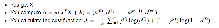
You will learn to:

• Build the general architecture of a learning algorithm, including:
  • Initializing parameters（初始化参数）
  • Calculating the cost function and its gradient（计算代价函数，和他的梯度）
  • Using an optimization algorithm (gradient descent)（使用梯度下降优化算法）
• Gather all three functions above into a main model function, in the right order.

1 - Packages（导入包，加载数据集）

其中，用到的Python包有：

• numpy 是使用Python进行科学计算的基础包。 
• h5py Python提供读取HDF5二进制数据格式文件的接口，本次的训练及测试图片集是以HDF5储存的。 
• matplotlib 是Python中著名的绘图库。 
• PIL (Python Image Library) 为 Python提供图像处理功能。 
• scipy 基于NumPy来做高等数学、信号处理、优化、统计和许多其它科学任务的拓展库。

import numpy as np
import matplotlib.pyplot as plt
import h5py
import scipy
from PIL import Image
from scipy import ndimage
from lr_utils import load_dataset   # 用来导入数据集的

%matplotlib inline   #设置matplotlib在行内显示图片

%load lr_utils.py， 如果该作业在本地运行，该代码保存在 lr_utils.py文件，和当前项目保存在一个文件夹下
import numpy as np
import h5py


def load_dataset():
    train_dataset = h5py.File('datasets/train_catvnoncat.h5', "r")
    train_set_x_orig = np.array(train_dataset["train_set_x"][:]) # your train set features
    train_set_y_orig = np.array(train_dataset["train_set_y"][:]) # your train set labels

    test_dataset = h5py.File('datasets/test_catvnoncat.h5', "r")
    test_set_x_orig = np.array(test_dataset["test_set_x"][:]) # your test set features
    test_set_y_orig = np.array(test_dataset["test_set_y"][:]) # your test set labels

    classes = np.array(test_dataset["list_classes"][:]) # the list of classes

    train_set_y_orig = train_set_y_orig.reshape((1, train_set_y_orig.shape[0]))
    test_set_y_orig = test_set_y_orig.reshape((1, test_set_y_orig.shape[0]))

    return train_set_x_orig, train_set_y_orig, test_set_x_orig, test_set_y_orig, classes

2 - Overview of the Problem set（目标：预处理数据）

Problem Statement: You are given a dataset ("data.h5") containing:

- a training set of m_train images labeled as cat (y=1) or non-cat (y=0)
- a test set of m_test images labeled as cat or non-cat
- each image is of shape (num_px, num_px, 3) where 3 is for the 3 channels (RGB). Thus, each image is square (height = num_px) and (width = num_px).

2.1 导入数据

# Loading the data (cat/non-cat)
train_set_x_orig, train_set_y, test_set_x_orig, test_set_y, classes = load_dataset()

2.2 熟悉数据

• 我们打算预处理这些数据，重新命名数据为 train_set_x, test_set_x。标签数据没必要预处理

• train_set_x 和 test_set_x 是一个数组，代表一个图像，你可以运行下面代码预览一个例子，也可以通过修改索引查看其它图片）

# Example of a picture
index = 25
plt.imshow(train_set_x_orig[index])
print ("y = " + str(train_set_y[:,index]) + ", it's a '" + classes[np.squeeze(train_set_y[:,index])].decode("utf-8") +  "' picture.")

y = [1], it's a 'cat' picture.

• 许多深度学习里的bug来自于矩阵/向量维度不匹配，如果你能保持你的矩阵/向量维度清晰，你可以消除很多bug

Exercise: Find the values for:

- m_train (number of training examples)
- m_test (number of test examples)
- num_px (= height = width of a training image)

• 计算训练集、测试集的大小以及图像的大小

### START CODE HERE ### (≈ 3 lines of code)
m_train = train_set_y.shape[1]
m_test = test_set_y.shape[1]
num_px = train_set_x_orig.shape[1]
### END CODE HERE ###

print ("Number of training examples: m_train = " + str(m_train))
print ("Number of testing examples: m_test = " + str(m_test))
print ("Height/Width of each image: num_px = " + str(num_px))
print ("Each image is of size: (" + str(num_px) + ", " + str(num_px) + ", 3)")
print ("train_set_x shape: " + str(train_set_x_orig.shape))
print ("train_set_y shape: " + str(train_set_y.shape))
print ("test_set_x shape: " + str(test_set_x_orig.shape))
print ("test_set_y shape: " + str(test_set_y.shape))

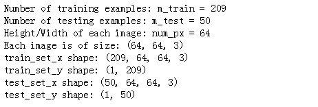
Expected Output for m_train, m_test and num_px:

m_train	209
m_test	50
num_px	64

 

2.3 转换矩阵

• 最终，整个训练集将会转为一个矩阵，其中包括num_px*num_py*3行，m_train列。

Exercise: Reshape the training and test data sets so that images of size (num_px, num_px, 3) are flattened into single vectors of shape (num_px ∗ num_px ∗ 3, 1).

其中X_flatten = X.reshape(X.shape[0], -1).T可以：将一个维度为(a,b,c,d)的矩阵转换为一个维度为(b∗c∗d, a)的矩阵。

• 转换图像为一个矢量，即矩阵的一列

X_flatten = X.reshape(X.shape[0], -1).T      # X.T is the transpose of X

# Reshape the training and test examples

### START CODE HERE ### (≈ 2 lines of code)
train_set_x_flatten = train_set_x_orig.reshape(train_set_x_orig.shape[0], -1).T
test_set_x_flatten = test_set_x_orig.reshape(test_set_x_orig.shape[0], -1).T

# 基础方法：需要的是 m_train 行 (shape[1]*shape[2]*shape[3]) 的数据, 所以需要转置，不知道为啥算出来和上面的方法不太一样。。。
# train_set_x_flatten = train_set_x_orig.reshape(train_set_x_orig.shape[1]*train_set_x_orig.shape[2]*train_set_x_orig.shape[3], train_set_x_orig.shape[0])
# test_set_x_flatten = test_set_x_orig.reshape(test_set_x_orig.shape[1]*test_set_x_orig.shape[2]*test_set_x_orig.shape[3], test_set_x_orig.shape[0])

### END CODE HERE ###
print ("train_set_x_flatten shape: " + str(train_set_x_flatten.shape))
print ("train_set_y shape: " + str(train_set_y.shape))
print ("test_set_x_flatten shape: " + str(test_set_x_flatten.shape))
print ("test_set_y shape: " + str(test_set_y.shape))
print ("sanity check after reshaping: " + str(train_set_x_flatten[0:5,0]))

# print ("sanity check after reshaping: " + str(train_set_x_flatten[:, :]))

Expected Output:

 

train_set_x_flatten shape	(12288, 209)
train_set_y shape	(1, 209)
test_set_x_flatten shape	(12288, 50)
test_set_y shape	(1, 50)
sanity check after reshaping	[17 31 56 22 33]

2.4 预处理数据（去中心化）

• 为了表示图像（RGB）必须指定为每个像素，实际上像素值就是三个数字组成的向量（0-255））
• 通常机器学习的预处理工作是 去中心化和标准化你的数据集， (x - mean)/标准差。但是对图像数据集，数据集的每一行除以255(最大值的像素通道）更简单方便高效）

train_set_x = train_set_x_flatten / 255.
test_set_x = test_set_x_flatten / 255.

What you need to remember:

常见的预处理一个新数据集的步骤是:

• Figure out the dimensions and shapes of the problem (m_train, m_test, num_px, ...)
• Reshape the datasets such that each example is now a vector of size (num_px * num_px * 3, 1)
• "Standardize" the data

3 - General Architecture of the learning algorithm（算法流程）

• 设计一个简单的算法来区分猫的猫图片的图像。
• 你将用神经网络的思想构建一个逻辑回归，下面的图像解释为什么逻辑回归实际上是一个非常简单神经网络！

 

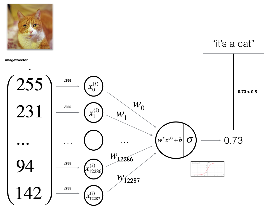
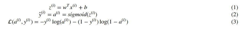
 算法的数学表达式：

对一个 样例 

计算所有训练样本代价：

Key steps: In this exercise, you will carry out the following steps:

初始化模型的参数
通过最小化代价来学习模型的参数
使用学习好的参数来进行预测（在测试集上）
分析结果并做总结

4 - Building the parts of our algorithm（构建算法的部分）

搭建一个神经网络的主要步骤：

1. 定义模型结构(例如输入特征的数量) 
2. 初始化模型的参数
3. 循环操作
   • 计算当前的 loss 值（前向传播）
   • 计算当前的梯度值（反向传播）
   • 更新参数，梯度下降算法

你通常分别构建1-3.并把他们集成到一个model()函数中。

4.1 - sigmod()函数实现

Exercise: 实现 sigmod() 函数, 你需要计算 sigmoid(wTx+b) 来进行预测

# GRADED FUNCTION: sigmoid

def sigmoid(z):
    """
    Compute the sigmoid of z

    Arguments:
    x -- A scalar or numpy array of any size.

    Return:
    s -- sigmoid(z)
    """

    ### START CODE HERE ### (≈ 1 line of code)
    s = 1 / (1 + np.exp(-z))
    ### END CODE HERE ###
    
    return s

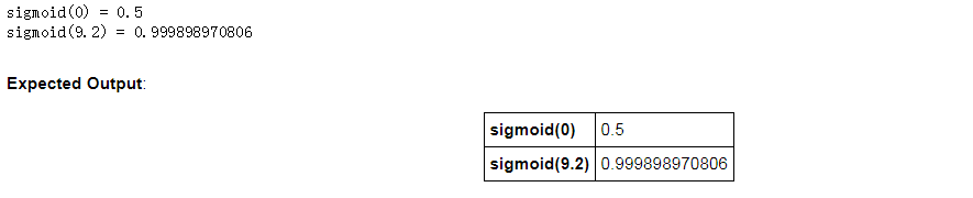
print ("sigmoid(0) = " + str(sigmoid(0)))
print ("sigmoid(9.2) = " + str(sigmoid(9.2)))

 

4.2 - 初始化参数（w,  b）

Exercise: 在下面实现参数初始化. 你不得不初始化 w 为一个零向量。使用 np.zeros().

# GRADED FUNCTION: initialize_with_zeros

def initialize_with_zeros(dim):
    """
    This function creates a vector of zeros of shape (dim, 1) for w and initializes b to 0.
    
    Argument:
    dim -- size of the w vector we want (or number of parameters in this case)
    
    Returns:
    w -- initialized vector of shape (dim, 1)
    b -- initialized scalar (corresponds to the bias)
    """
    
    ### START CODE HERE ### (≈ 1 line of code)
    w = np.zeros(shape=(dim, 1))      # 初始化 w 为 (dim行，1列) 的向量
    b = 0
    ### END CODE HERE ###

    assert(w.shape == (dim, 1))    # 判断 w 的shape是否为 (dim, 1), 不是则终止程序
    assert(isinstance(b, float) or isinstance(b, int))   # 判断 b 是否是float或者int类型
    
    return w, b

Expected Output:

w	[[ 0.] [ 0.]]
b	0

对于图像输入，w的维度是 (num_px * num_px * 3, 1)。

4.3 - 前向传播 和 后向传播

现在你的参数已经初始化，可以进行 前向传播 和 后向传播 步骤来学习参数。

Exercise: 实现一个函数  propagate() 来计算 代价函数 和 他的梯度

Hints：

Forward Propagation:

Here are the two formulas you will be using:

 

 

 

 

 

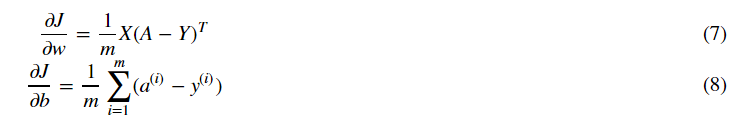
# GRADED FUNCTION: propagate

def propagate(w, b, X, Y):
    """
    Implement the cost function and its gradient for the propagation explained above

    Arguments:
    w -- weights, a numpy array of size (num_px * num_px * 3, 1)
    b -- bias, a scalar
    X -- data of size (num_px * num_px * 3, number of examples)
    Y -- true "label" vector (containing 0 if non-cat, 1 if cat) of size (1, number of examples)

    Return:
    cost -- negative log-likelihood cost for logistic regression
    dw -- gradient of the loss with respect to w, thus same shape as w
    db -- gradient of the loss with respect to b, thus same shape as b
    
    Tips:
    - Write your code step by step for the propagation
    """
    
    m = X.shape[1]      # 样例数
#     print(m)
    
    # 前向传播(Forward Propagation) (FROM X TO COST)
    ### START CODE HERE ### (≈ 2 lines of code)
    
    A = sigmoid(np.dot(w.T, X) + b) # 计算 activation , A 的 维度是 (m, m)
    cost = (- 1 / m) * np.sum(Y * np.log(A) + (1 - Y) * (np.log(1 - A)))  # 计算 cost; Y == yhat(1, m)

    ### END CODE HERE ###
    
    # 反向传播(Backward Propagation) (TO FIND GRAD)
    ### START CODE HERE ### (≈ 2 lines of code)
    
    dw = (1 / m) * np.dot(X, (A - Y).T)   # 计算 w 的导数
    db = (1 / m) * np.sum(A - Y)          # 计算 b 的导数
    
    ### END CODE HERE ###

    assert(dw.shape == w.shape)          # 这些代码 会 减少bug出现
    assert(db.dtype == float)            # db 是一个值
    cost = np.squeeze(cost)              # 压缩维度,(从数组的形状中删除单维条目，即把shape中为1的维度去掉)，保证cost是值
    assert(cost.shape == ())
    
    grads = {"dw": dw,
             "db": db}
    
    return grads, cost

w, b, X, Y = np.array([[1], [2]]), 2, np.array([[1,2], [3,4]]), np.array([[1, 0]])
grads, cost = propagate(w, b, X, Y) 
print ("dw = " + str(grads["dw"]))  
print ("db = " + str(grads["db"]))  
print ("cost = " + str(cost))

 

Expected Output:

dw	[[ 0.99993216] [ 1.99980262]]
db	0.499935230625
cost	6.000064773192205

4.4 Optimization(最优化)

• 你已经初始化了你的参数。
• 你已经能够计算一个代价函数和他的梯度。
• 现在，你需要用梯度下降算法更新参数。

 Exercise: 写下 optimization function（优化函数），目标是通过最小化代价函数 J，学习参数 w 和 b。对参数 θ，更新规则是 θ = θ - α dθ，α是 learning rate）

# GRADED FUNCTION: optimize

def optimize(w, b, X, Y, num_iterations, learning_rate, print_cost = False):
    """
    This function optimizes w and b by running a gradient descent algorithm
    
    Arguments:
    w -- weights, a numpy array of size (num_px * num_px * 3, 1)
    b -- bias, a scalar
    X -- data of shape (num_px * num_px * 3, number of examples)
    Y -- true "label" vector (containing 0 if non-cat, 1 if cat), of shape (1, number of examples)
    num_iterations -- number of iterations of the optimization loop
    learning_rate -- learning rate of the gradient descent update rule
    print_cost -- True to print the loss every 100 steps
    
    Returns:
    params -- dictionary containing the weights w and bias b
    grads -- dictionary containing the gradients of the weights and bias with respect to the cost function
    costs -- list of all the costs computed during the optimization, this will be used to plot the learning curve.
    
    Tips:
    You basically need to write down two steps and iterate through them:
        1) Calculate the cost and the gradient for the current parameters. Use propagate().
        2) Update the parameters using gradient descent rule for w and b.
    """
    
    costs = []
    
    for i in range(num_iterations):
        
        
        # Cost and gradient calculation
        ### START CODE HERE ###       
        grads, cost = propagate(w, b, X, Y)     
        ### END CODE HERE ###
        
        # Retrieve derivatives from grads(获取导数)
        dw = grads["dw"]
        db = grads["db"]
        
        # update rule (更新 参数)
        ### START CODE HERE ###
        w = w - learning_rate * dw  # need to broadcast
        b = b - learning_rate * db      
        ### END CODE HERE ###
        
        # Record the costs (每一百次记录一次 cost)
        if i % 100 == 0:
            costs.append(cost)
        
        # Print the cost every 100 training examples (如果需要打印则每一百次打印一次)
        if print_cost and i % 100 == 0:
            print ("Cost after iteration %i: %f" % (i, cost))
    
    # 记录 迭代好的参数 (w, b)
    params = {"w": w,
              "b": b}
    
    # 记录当前导数(dw, db), 以便下次继续迭代
    grads = {"dw": dw,
             "db": db}
    
    return params, grads, costs

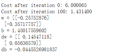
params, grads, costs = optimize(w, b, X, Y, num_iterations= 200, learning_rate = 0.009, print_cost = True)

print ("w = " + str(params["w"]))
print ("b = " + str(params["b"]))
print ("dw = " + str(grads["dw"]))
print ("db = " + str(grads["db"]))

Exercise: 前面的函数 将输出学习好的参数 (w, b), 我们可以使用w和b来预测数据集 x 的标签，实现 predict() 函数。计算预测有两个步骤：

1. 计算 Y_hat = A = sigmod(w.T X + b)
2. 转换 a 为 0 (如果 activation <= 0.5) 或者 1 (如果activation > 0.5)，存储预测值在 向量Y_prediction中。如果你想，你可以在for循环中使用 if/else（尽管有方法将其向量化）

# GRADED FUNCTION: predict

def predict(w, b, X):
    '''
    Predict whether the label is 0 or 1 using learned logistic regression parameters (w, b)
    
    Arguments:
    w -- weights, a numpy array of size (num_px * num_px * 3, 1)
    b -- bias, a scalar
    X -- data of size (num_px * num_px * 3, number of examples)
    
    Returns:
    Y_prediction -- a numpy array (vector) containing all predictions (0/1) for the examples in X
    '''
    
    m = X.shape[1]
    Y_prediction = np.zeros((1, m))
    w = w.reshape(X.shape[0], 1)
    
    # Compute vector "A" predicting the probabilities of a cat being present in the picture
    ### START CODE HERE ### (≈ 1 line of code)
    A = sigmoid(np.dot(w.T, X) + b)
    ### END CODE HERE ###
    
    for i in range(A.shape[1]):
        # Convert probabilities a[0,i] to actual predictions p[0,i]
        ### START CODE HERE ### (≈ 4 lines of code)
        Y_prediction[0, i] = 1 if A[0, i] > 0.5 else 0
        ### END CODE HERE ###
    
    assert(Y_prediction.shape == (1, m))
    
    return Y_prediction

print("predictions = " + str(predict(w, b, X))) 

Expected Output:

predictions

[[ 1. 1.]]

What to remember: You've implemented several functions that:

• 初始化参数 (w, b)
• 迭代优化 损失值 以学习参数(w，b) ：
  • 计算 代价值 和 他的梯度
  • 用梯度下降算法更新参数
• 使用学习好的(w, b)来进行预测给定的 样本集标签

5 - 合并所有函数在一个model()里

你将看到如何通过将所有构建（在前面部分中实现的功能）按照正确的顺序组合在一起来构建整个模型。

Exercise: Implement the model function. Use the following notation:

• Y_prediction ：你在测试集上进行预测
• Y_prediction_train：你在训练集上的预测
• w, costs, grads ：optimize()的输出

# GRADED FUNCTION: model

def model(X_train, Y_train, X_test, Y_test, num_iterations=2000, learning_rate=0.5, print_cost=False):
    """
    Builds the logistic regression model by calling the function you've implemented previously
    
    Arguments:
    X_train -- training set represented by a numpy array of shape (num_px * num_px * 3, m_train)
    Y_train -- training labels represented by a numpy array (vector) of shape (1, m_train)
    X_test -- test set represented by a numpy array of shape (num_px * num_px * 3, m_test)
    Y_test -- test labels represented by a numpy array (vector) of shape (1, m_test)
    num_iterations -- hyperparameter representing the number of iterations to optimize the parameters
    learning_rate -- hyperparameter representing the learning rate used in the update rule of optimize()
    print_cost -- Set to true to print the cost every 100 iterations
    
    Returns:
    d -- dictionary containing information about the model.
    """
    
    ### START CODE HERE ###
    # initialize parameters with zeros (初始化参数(w, b))
    w, b = initialize_with_zeros(X_train.shape[0])         # num_px*num_px*3

    # Gradient descent (前向传播和后向传播 同时 梯度下降更新参数)
    parameters, grads, costs = optimize(w, b, X_train, Y_train, num_iterations, learning_rate, print_cost)
    
    # Retrieve parameters w and b from dictionary "parameters"(获取参数w, b)
    w = parameters["w"]
    b = parameters["b"]
    
    # Predict test/train set examples (使用测试集和训练集进行预测)
    Y_prediction_test = predict(w, b, X_test)
    Y_prediction_train = predict(w, b, X_train)

    ### END CODE HERE ###

    # Print train/test Errors (训练/测试误差: (100 - mean(abs(Y_hat - Y))*100 )
    print("train accuracy: {} %".format(100 - np.mean(np.abs(Y_prediction_train - Y_train)) * 100))
    print("test accuracy: {} %".format(100 - np.mean(np.abs(Y_prediction_test - Y_test)) * 100))

    
    d = {"costs": costs,
         "Y_prediction_test": Y_prediction_test, 
         "Y_prediction_train" : Y_prediction_train, 
         "w" : w, 
         "b" : b,
         "learning_rate" : learning_rate,
         "num_iterations": num_iterations}
    
    return d

d = model(train_set_x, train_set_y, test_set_x, test_set_y, num_iterations = 2000, learning_rate = 0.005, print_cost = True)

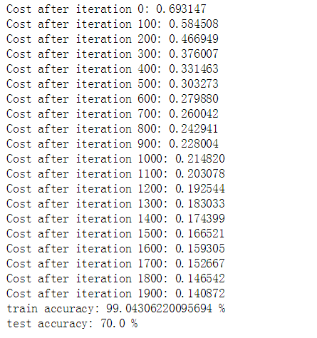
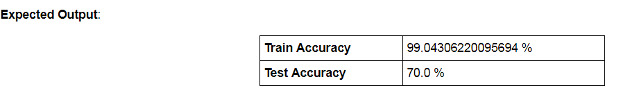
Comment: 训练集准确率接近 100%. 这是一个很好的检查：你的模型能够工作，并且有足够能力去拟合训练数据。 鉴于我们使用的小数据集和逻辑回归是一个线性分类器，测试误差 是 68%，这对这样简单的模型来说还不坏。

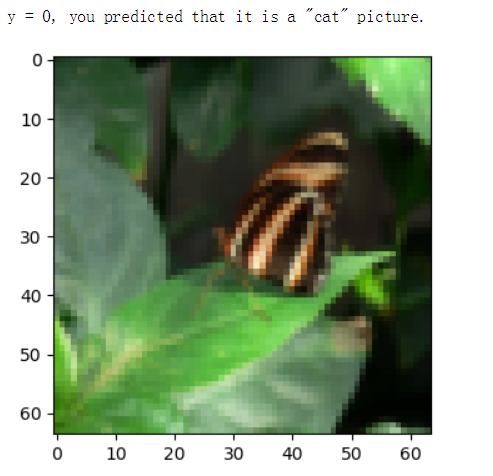
此为，你还可以看到，该模型显然对培训数据进行了过渡拟合。在这个专门化后面，你将学习如何减少过渡拟合。例如通过使用 正则化。使用下面的代码（更改索引变量），你可以查看测试集上图片的预测。

 

# Example of a picture that was wrongly classified.
index = 5

plt.imshow(test_set_x[:,index].reshape((num_px, num_px, 3)))

# test_set_y[0, index]：测试集里标签;  classes[int(d["Y_Prediction_test"][0, index])]：预测值
print ("y = " + str(test_set_y[0, index]) + ", you predicted that it is a \"" + 
       classes[int(d["Y_prediction_test"][0, index])].decode("utf-8") +  "\" picture.")

 

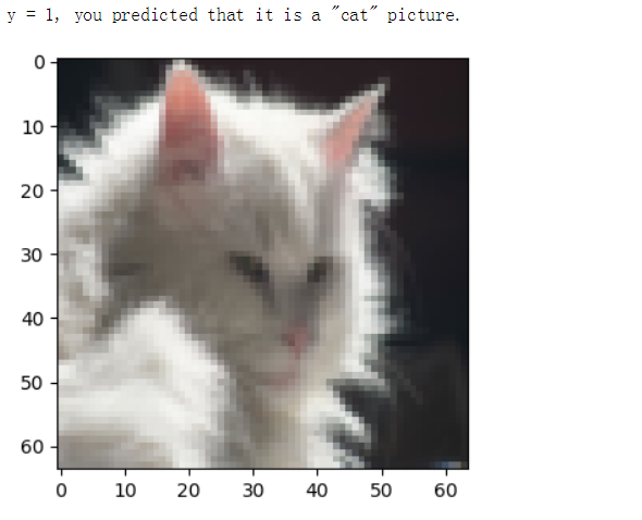
精确性不是很高。。。

 

# Plot learning curve (with costs)
costs = np.squeeze(d['costs'])
plt.plot(costs)
plt.ylabel('cost')
plt.xlabel('iterations (per hundreds)')
plt.title("Learning rate =" + str(d["learning_rate"]))
plt.show()

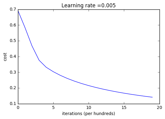
Interpretation: 你可以看见成本在下降。这表明参数正则学习中。但是你可以看到，你可以在训练集对模型进行更多的培训。尝试增加以上代码中的迭代次数，并重新运行代码。你会看见，训练集的准确性会提高，但是测试集的精度会下降。这就是过渡拟合。

6 - Further analysis 

检查 learning rate α.的可能选择

选择一个learning rate α

Reminder：为了让梯度下降能够工作，你必须明智的选择learning rate α。α决定了我们更新参数的速度。如果学习率太高，我们可能会”超过”最优值。同样，如果他太小，我们将需要太多的迭代来收敛到最佳值。这就是为什么使用良好α至关重要。

让我们比较我们的模型的α与几种选择的α。

learning_rates = [0.01, 0.001, 0.0001]
models = {}
for i in learning_rates:
    print ("learning rate is: " + str(i))
    models[str(i)] = model(train_set_x, train_set_y, test_set_x, test_set_y, num_iterations = 1500, learning_rate = i, print_cost = False)
    print ('\n' + "-------------------------------------------------------" + '\n')

for i in learning_rates:
    plt.plot(np.squeeze(models[str(i)]["costs"]), label= str(models[str(i)]["learning_rate"]))

plt.ylabel('cost')
plt.xlabel('iterations')

legend = plt.legend(loc='upper center', shadow=True)
frame = legend.get_frame()
frame.set_facecolor('0.90')
plt.show()

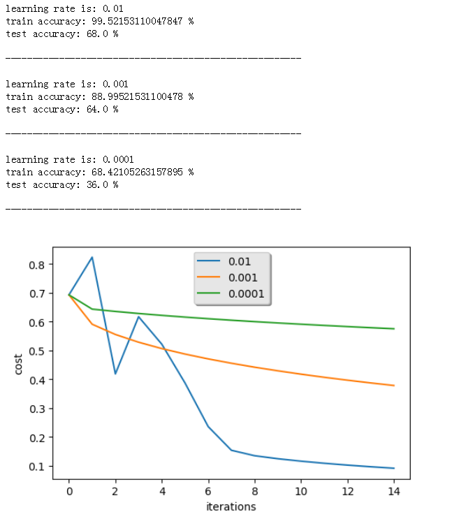
Interpretation:

• 不同α带来不同的cost，因此不同预测结果
• 如果学习率太高(0.01)，cost可能上下波。(尽管本例中0.01还行)
• 更低的成本不意味着一个更好的模型。你需要检查一下是否可能过拟合。当训练精度远远高于测试精度时，就会过拟合！
• 在深度学习中，我们推荐
• 选择能够更好最小化代价的 learning rate
• 如果模型过拟合，选择其他技术减少过拟合，后面会讲！

7 - Test with your own image

你可以使用 你的图片 来测试 你的模型的输出。.做这些：

 

import imageio
from skimage.transform import resize

## START CODE HERE ## (PUT YOUR IMAGE NAME) 
my_image = "my_image4.jpg"   # 修改你图像的名字
## END CODE HERE ##

# We preprocess the image to fit your algorithm.
fname = "images/" + my_image                              # 图片位置     
image = np.array(imageio.imread(fname))                   # 读入图片为矩阵, 这里用原版本的会出错，scipy的那个函数被删了
print(image.shape)

# 转置图片为 (num_px*num_px*3, 1)向量
my_image = resize(image, output_shape=(num_px, num_px)).reshape((1, num_px * num_px * 3)).T
print(my_image)

my_predicted_image = predict(d["w"], d["b"], my_image)  # 用训练好的参数来预测图像

plt.imshow(image)

print(classes)
print("y = " + str(np.squeeze(my_predicted_image)) + ", your algorithm predicts a \"" + classes[int(np.squeeze(my_predicted_image)),].decode("utf-8") +  "\" picture.")

 

y = 1.0, your algorithm predicts a "cat" picture.

What to remember from this assignment:

• 预处理你的数据集很重要Preprocessing the dataset is important.
• 你分别实现每个函数: initialize(), propagate(), optimize(). 然后你整合成 一个 model().
• 调整你的learning rate (which is an example of a "hyperparameter") 可以对算法产生很大的影响. 

 

代码综合

import numpy as np
import matplotlib.pyplot as plt
import h5py
import scipy
from PIL import Image
from scipy import ndimage
from lr_utils import load_dataset   # 用来导入数据集的

import skimage

%matplotlib inline


# Loading the data (cat/non-cat)
train_set_x_orig, train_set_y, test_set_x_orig, test_set_y, classes = load_dataset()



### START CODE HERE ### (≈ 3 lines of code)
m_train = train_set_y.shape[1]   # or train_set_x_orig.shape[0]
m_test = test_set_y.shape[1]
num_px = train_set_x_orig.shape[1]

### END CODE HERE ###

print ("Number of training examples: m_train = " + str(m_train))
print ("Number of testing examples: m_test = " + str(m_test))
print ("Height/Width of each image: num_px = " + str(num_px))
print ("Each image is of size: (" + str(num_px) + ", " + str(num_px) + ", 3)")
print ("train_set_x shape: " + str(train_set_x_orig.shape))
print ("train_set_y shape: " + str(train_set_y.shape))
print ("test_set_x shape: " + str(test_set_x_orig.shape))
print ("test_set_y shape: " + str(test_set_y.shape))



# Reshape the training and test examples

### START CODE HERE ### (≈ 2 lines of code)
train_set_x_flatten = train_set_x_orig.reshape(train_set_x_orig.shape[0], -1).T
test_set_x_flatten = test_set_x_orig.reshape(test_set_x_orig.shape[0], -1).T

### END CODE HERE ###
print ("train_set_x_flatten shape: " + str(train_set_x_flatten.shape))
print ("train_set_y shape: " + str(train_set_y.shape))
print ("test_set_x_flatten shape: " + str(test_set_x_flatten.shape))
print ("test_set_y shape: " + str(test_set_y.shape))
print ("sanity check after reshaping: " + str(train_set_x_flatten[0:5,0]))


train_set_x = train_set_x_flatten / 255.
test_set_x = test_set_x_flatten / 255.



# GRADED FUNCTION: sigmoid

def sigmoid(z):
    """
    Compute the sigmoid of z

    Arguments:
    x -- A scalar or numpy array of any size.

    Return:
    s -- sigmoid(z)
    """

    ### START CODE HERE ### (≈ 1 line of code)
    s = 1 / (1 + np.exp(-z))
    ### END CODE HERE ###
    
    return s


# GRADED FUNCTION: initialize_with_zeros
def initialize_with_zeros(dim):
    """
    This function creates a vector of zeros of shape (dim, 1) for w and initializes b to 0.
    
    Argument:
    dim -- size of the w vector we want (or number of parameters in this case)
    
    Returns:
    w -- initialized vector of shape (dim, 1)
    b -- initialized scalar (corresponds to the bias)
    """
    
    ### START CODE HERE ### (≈ 1 line of code)
    w = np.zeros(shape=(dim, 1))
    b = 0
    ### END CODE HERE ###

    assert(w.shape == (dim, 1))    # 判断 w 的shape是否为 (dim, 1), 不是则终止程序
    assert(isinstance(b, float) or isinstance(b, int))   # 判断 b 是否是float或者int类型
    
    return w, b



# GRADED FUNCTION: propagate

def propagate(w, b, X, Y):
    """
    Implement the cost function and its gradient for the propagation explained above

    Arguments:
    w -- weights, a numpy array of size (num_px * num_px * 3, 1)
    b -- bias, a scalar
    X -- data of size (num_px * num_px * 3, number of examples)
    Y -- true "label" vector (containing 0 if non-cat, 1 if cat) of size (1, number of examples)

    Return:
    cost -- negative log-likelihood cost for logistic regression
    dw -- gradient of the loss with respect to w, thus same shape as w
    db -- gradient of the loss with respect to b, thus same shape as b
    
    Tips:
    - Write your code step by step for the propagation
    """
    
    m = X.shape[1]      # 样例数
#     print(m)
    
    # 前向传播(Forward Propagation) (FROM X TO COST)
    ### START CODE HERE ### (≈ 2 lines of code)
    
    A = sigmoid(np.dot(w.T, X) + b) # 计算 activation , A 的 维度是 (m, m)
    cost = (- 1 / m) * np.sum(Y * np.log(A) + (1 - Y) * (np.log(1 - A)))  # 计算 cost; Y == yhat(1, m)

    ### END CODE HERE ###
    
    # 反向传播(Backward Propagation) (TO FIND GRAD)
    ### START CODE HERE ### (≈ 2 lines of code)
    
    dw = (1 / m) * np.dot(X, (A - Y).T)   # 计算 w 的导数
    db = (1 / m) * np.sum(A - Y)          # 计算 b 的导数
    
    ### END CODE HERE ###

    assert(dw.shape == w.shape)          # 这些代码 会 减少bug出现
    assert(db.dtype == float)            # db 是一个值
    cost = np.squeeze(cost)              # 压缩维度,(从数组的形状中删除单维条目，即把shape中为1的维度去掉)
    assert(cost.shape == ())
    
    grads = {"dw": dw,
             "db": db}
    
    return grads, cost



# GRADED FUNCTION: optimize

def optimize(w, b, X, Y, num_iterations, learning_rate, print_cost = False):
    """
    This function optimizes w and b by running a gradient descent algorithm
    
    Arguments:
    w -- weights, a numpy array of size (num_px * num_px * 3, 1)
    b -- bias, a scalar
    X -- data of shape (num_px * num_px * 3, number of examples)
    Y -- true "label" vector (containing 0 if non-cat, 1 if cat), of shape (1, number of examples)
    num_iterations -- number of iterations of the optimization loop
    learning_rate -- learning rate of the gradient descent update rule
    print_cost -- True to print the loss every 100 steps
    
    Returns:
    params -- dictionary containing the weights w and bias b
    grads -- dictionary containing the gradients of the weights and bias with respect to the cost function
    costs -- list of all the costs computed during the optimization, this will be used to plot the learning curve.
    
    Tips:
    You basically need to write down two steps and iterate through them:
        1) Calculate the cost and the gradient for the current parameters. Use propagate().
        2) Update the parameters using gradient descent rule for w and b.
    """
    
    costs = []
    
    for i in range(num_iterations):
        
        
        # Cost and gradient calculation
        ### START CODE HERE ###       
        grads, cost = propagate(w, b, X, Y)     
        ### END CODE HERE ###
        
        # Retrieve derivatives from grads(获取导数)
        dw = grads["dw"]
        db = grads["db"]
        
        # update rule (更新 参数)
        ### START CODE HERE ###
        w = w - learning_rate * dw  # need to broadcast
        b = b - learning_rate * db      
        ### END CODE HERE ###
        
        # Record the costs (每一百次记录一次 cost)
        if i % 100 == 0:
            costs.append(cost)
        
        # Print the cost every 100 training examples (如果需要打印则每一百次打印一次)
        if print_cost and i % 100 == 0:
            print ("Cost after iteration %i: %f" % (i, cost))
    
    # 记录 迭代好的参数 (w, b)
    params = {"w": w,
              "b": b}
    
    # 记录当前导数(dw, db), 以便下次继续迭代
    grads = {"dw": dw,
             "db": db}
    
    return params, grads, costs





# GRADED FUNCTION: predict

def predict(w, b, X):
    '''
    Predict whether the label is 0 or 1 using learned logistic regression parameters (w, b)
    
    Arguments:
    w -- weights, a numpy array of size (num_px * num_px * 3, 1)
    b -- bias, a scalar
    X -- data of size (num_px * num_px * 3, number of examples)
    
    Returns:
    Y_prediction -- a numpy array (vector) containing all predictions (0/1) for the examples in X
    '''
    
    m = X.shape[1]
    Y_prediction = np.zeros((1, m))
    w = w.reshape(X.shape[0], 1)
    
    # Compute vector "A" predicting the probabilities of a cat being present in the picture
    ### START CODE HERE ### (≈ 1 line of code)
    A = sigmoid(np.dot(w.T, X) + b)
    ### END CODE HERE ###
    
    for i in range(A.shape[1]):
        # Convert probabilities a[0,i] to actual predictions p[0,i]
        ### START CODE HERE ### (≈ 4 lines of code)
        Y_prediction[0, i] = 1 if A[0, i] > 0.5 else 0
        ### END CODE HERE ###
    
    assert(Y_prediction.shape == (1, m))
    
    return Y_prediction



# GRADED FUNCTION: model

def model(X_train, Y_train, X_test, Y_test, num_iterations=2000, learning_rate=0.5, print_cost=False):
    """
    Builds the logistic regression model by calling the function you've implemented previously
    
    Arguments:
    X_train -- training set represented by a numpy array of shape (num_px * num_px * 3, m_train)
    Y_train -- training labels represented by a numpy array (vector) of shape (1, m_train)
    X_test -- test set represented by a numpy array of shape (num_px * num_px * 3, m_test)
    Y_test -- test labels represented by a numpy array (vector) of shape (1, m_test)
    num_iterations -- hyperparameter representing the number of iterations to optimize the parameters
    learning_rate -- hyperparameter representing the learning rate used in the update rule of optimize()
    print_cost -- Set to true to print the cost every 100 iterations
    
    Returns:
    d -- dictionary containing information about the model.
    """
    
    ### START CODE HERE ###
    # initialize parameters with zeros (初始化参数(w, b))
    w, b = initialize_with_zeros(X_train.shape[0])         # num_px*num_px*3

    # Gradient descent (前向传播和后向传播 同时 梯度下降更新参数)
    parameters, grads, costs = optimize(w, b, X_train, Y_train, num_iterations, learning_rate, print_cost)
    
    # Retrieve parameters w and b from dictionary "parameters"(获取参数w, b)
    w = parameters["w"]
    b = parameters["b"]
    
    # Predict test/train set examples (使用测试集和训练集进行预测)
    Y_prediction_test = predict(w, b, X_test)
    Y_prediction_train = predict(w, b, X_train)

    ### END CODE HERE ###

    # Print train/test Errors (训练/测试误差: (100 - mean(abs(Y_hat - Y))*100 )
    print("train accuracy: {} %".format(100 - np.mean(np.abs(Y_prediction_train - Y_train)) * 100))
    print("test accuracy: {} %".format(100 - np.mean(np.abs(Y_prediction_test - Y_test)) * 100))

    
    d = {"costs": costs,
         "Y_prediction_test": Y_prediction_test, 
         "Y_prediction_train" : Y_prediction_train, 
         "w" : w, 
         "b" : b,
         "learning_rate" : learning_rate,
         "num_iterations": num_iterations}
    
    return d


d = model(train_set_x, train_set_y, test_set_x, test_set_y, num_iterations = 2000, learning_rate = 0.005, print_cost = True)


# Example of a picture that was wrongly classified.
index = 24

plt.imshow(test_set_x[:,index].reshape((num_px, num_px, 3)))

# test_set_y[0, index]：测试集里标签;  classes[int(d["Y_Prediction_test"][0, index])]：预测值
print ("y = " + str(test_set_y[0, index]) + ", you predicted that it is a \"" + 
       classes[int(d["Y_prediction_test"][0, index])].decode("utf-8") +  "\" picture.")