seaborn基本使用(二)

客户贷款风险评估

数据预处理

# 因为需要进行聚类，所以需要对数据进行初步处理，这里对数值型数据，进行标准化，对分类变量处理为有序变量。
# 选择特征   把文本类型转化为数值类型 方便计算比较 数据预处理
features = ['Age', 'Sex', 'Job', 'Housing', 'Saving accounts', 'Checking account', 'Credit amount', 'Duration']
new_data = data[features].copy()
 
# 对类别型特征进行有序编码
new_data['Sex'] = new_data['Sex'].map({
    'female': 0,
    'male': 1})
 
new_data['Housing'] = new_data['Housing'].map({
    'free': 0,
    'rent': 1,
    'own': 2})
# 这行代码的作用是将 'Housing' 列中的字符串值 'free' 替换为 0，'rent' 替换为 1，'own' 替换为 2。这种操作通常用于将分类变量（categorical variable）转换为数值型变量，以便在机器学习模型中使用。
 
# 'Housing' 列的字符串值被映射为相应的数字
new_data['Saving accounts'] = new_data['Saving accounts'].map({
    'unknown': 0,
    'little': 1,
    # 'moderate': 2,
    'quite rich': 3,
    'rich': 4})
 
new_data['Checking account'] = new_data['Checking account'].map({
    'unknown': 0,
    'little': 1,
    'moderate': 2,
    'rich': 3})
 
# 标准化数值型特征  正则化   标准正态分布
scaler = StandardScaler()
num_features = ['Age', 'Credit amount', 'Duration']
new_data[num_features] = scaler.fit_transform(new_data[num_features])
 
print(new_data.head(10))
 
# 划分高风险客户和低风险客户
 
# 假设 df 是你的 DataFrame，'column_name' 是要处理的列名
new_data['Age'] = new_data['Age'].round(2)
new_data['Duration'] = new_data['Duration'].round(2)
new_data['Credit amount'] = new_data['Credit amount'].round(2)
new_data['Saving accounts'].fillna(0, inplace=True)
print("整理后查看各列缺失值",new_data.isna().sum())
# 假设 df 是你的 DataFrame
new_data.to_csv('./out/output_new_data.csv', index=False)

查看详情

• 控制台打印

        Age  Sex  Job  ...  Checking account  Credit amount  Duration
0  2.766456    1    2  ...                 1      -0.745131 -1.236478
1 -1.191404    0    2  ...                 2       0.949817  2.248194
2  1.183312    1    1  ...                 0      -0.416562 -0.738668
3  0.831502    1    2  ...                 1       1.634247  1.750384
4  1.535122    1    2  ...                 1       0.566664  0.256953
5 -0.048022    1    1  ...                 0       2.050009  1.252574
6  1.535122    1    2  ...                 0      -0.154629  0.256953
7 -0.048022    1    3  ...                 2       1.303197  1.252574
8  2.238742    1    1  ...                 0      -0.075233 -0.738668
9 -0.663689    1    3  ...                 2       0.695681  0.754763
 
[10 rows x 8 columns]
整理后查看各列缺失值 Age                 0
Sex                 0
Job                 0
Housing             0
Saving accounts     0
Checking account    0
Credit amount       0
Duration            0
dtype: int64

案例1

# 导入需要的库
import pandas as pd
import numpy as np
import seaborn as sns
import matplotlib.pyplot as plt
from sklearn.preprocessing import StandardScaler
from sklearn.cluster import KMeans
from sklearn.metrics import silhouette_score
from sklearn.model_selection import train_test_split
from sklearn.utils import resample
from sklearn.ensemble import RandomForestClassifier
from sklearn.metrics import classification_report,confusion_matrix
new_data = pd.read_csv("./out/output_new_data.csv")
data = pd.read_csv("./german_credit_data.csv")
# 模型选择：使用KMeans进行聚类
kmeans = KMeans(n_clusters=2, random_state=15)
from sklearn.cluster import KMeans
# 检查无穷大值： 使用 Pandas 的 replace() 方法，可以将无穷大值替换为其他值。
new_data.replace([np.inf, -np.inf], np.nan, inplace=True)
print(new_data.describe(include='all'))
clusters = kmeans.fit_predict(new_data)
# 将聚类结果添加到数据中
data['Risk Group'] = clusters
print(data.head(10))
 
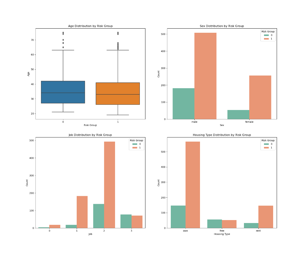
# 6.3两类客户之间对比
# 6.3.1基本情况对比
fig, axs = plt.subplots(2, 2, figsize=(18,15))
 
sns.boxplot(x='Risk Group', y='Age', data=data, ax=axs[0, 0])
axs[0, 0].set_title('Age Distribution by Risk Group')
axs[0, 0].set_xlabel('Risk Group')
axs[0, 0].set_ylabel('Age')
#
sns.countplot(x='Sex', hue='Risk Group', data=data, palette='Set2', ax=axs[0, 1])
axs[0, 1].set_title('Sex Distribution by Risk Group')
axs[0, 1].set_xlabel('Sex')
axs[0, 1].set_ylabel('Count')
 
sns.countplot(x='Job', hue='Risk Group', data=data, palette='Set2', ax=axs[1, 0])
axs[1, 0].set_title('Job Distribution by Risk Group')
axs[1, 0].set_xlabel('Job')
axs[1, 0].set_ylabel('Count')
 
sns.countplot(x='Housing', hue='Risk Group', data=data, palette='Set2', ax=axs[1, 1])
axs[1, 1].set_title('Housing Type Distribution by Risk Group')
axs[1, 1].set_xlabel('Housing Type')
axs[1, 1].set_ylabel('Count')
 
plt.show()

查看详情

• 控制台打印

               Age          Sex  ...  Credit amount    Duration
count  1000.000000  1000.000000  ...    1000.000000  1000.00000
mean     -0.000080     0.690000  ...      -0.000120    -0.00004
std       1.000554     0.462725  ...       1.000532     1.00074
min      -1.460000     0.000000  ...      -1.070000    -1.40000
25%      -0.750000     0.000000  ...      -0.680000    -0.74000
50%      -0.220000     1.000000  ...      -0.340000    -0.24000
75%       0.570000     1.000000  ...       0.250000     0.26000
max       3.470000     1.000000  ...       5.370000     4.24000
 
[8 rows x 8 columns]
   Id  Age     Sex  ...  Duration              Purpose Risk Group
0   0   67    male  ...         6             radio/TV          1
1   1   22  female  ...        48             radio/TV          0
2   2   49    male  ...        12            education          1
3   3   45    male  ...        42  furniture/equipment          0
4   4   53    male  ...        24                  car          0
5   5   35    male  ...        36            education          0
6   6   53    male  ...        24  furniture/equipment          1
7   7   35    male  ...        36                  car          0
8   8   61    male  ...        12             radio/TV          1
9   9   28    male  ...        30                  car          0

• 输出
  

案例2

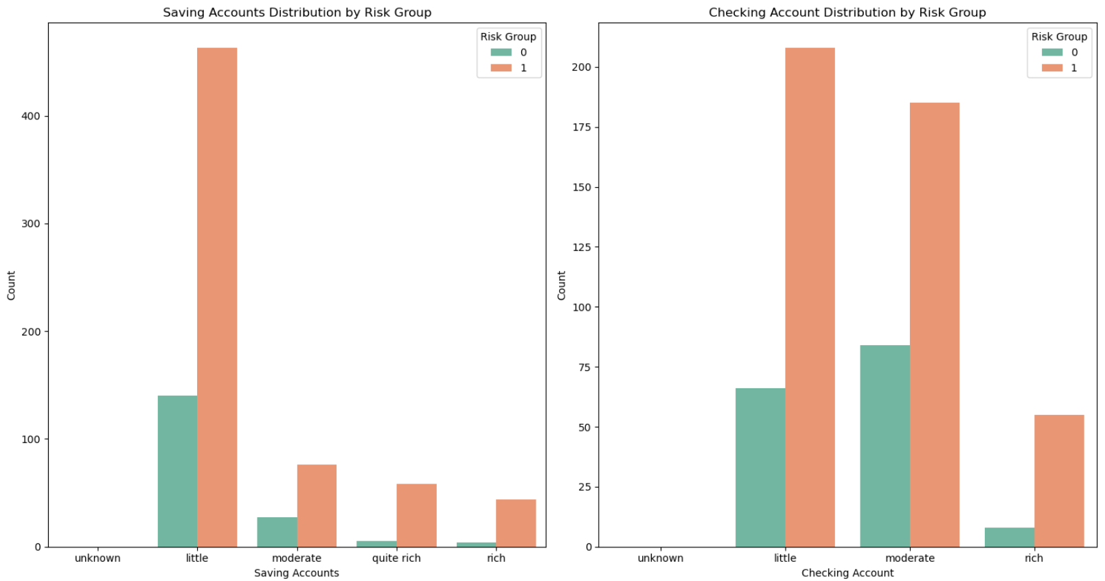
# 经济情况对比
order_savings = ['unknown', 'little', 'moderate', 'quite rich', 'rich']
order_checking = ['unknown', 'little', 'moderate', 'rich']
 
fig, axs = plt.subplots(1, 2, figsize=(15,8))
 
sns.countplot(x='Saving accounts', hue='Risk Group', data=data, order=order_savings, palette='Set2', ax=axs[0])
axs[0].set_title('Saving Accounts Distribution by Risk Group')
axs[0].set_xlabel('Saving Accounts')
axs[0].set_ylabel('Count')
 
sns.countplot(x='Checking account', hue='Risk Group', data=data, order=order_checking, palette='Set2', ax=axs[1])
axs[1].set_title('Checking Account Distribution by Risk Group')
axs[1].set_xlabel('Checking Account')
axs[1].set_ylabel('Count')
 
plt.tight_layout()
plt.show()

查看详情

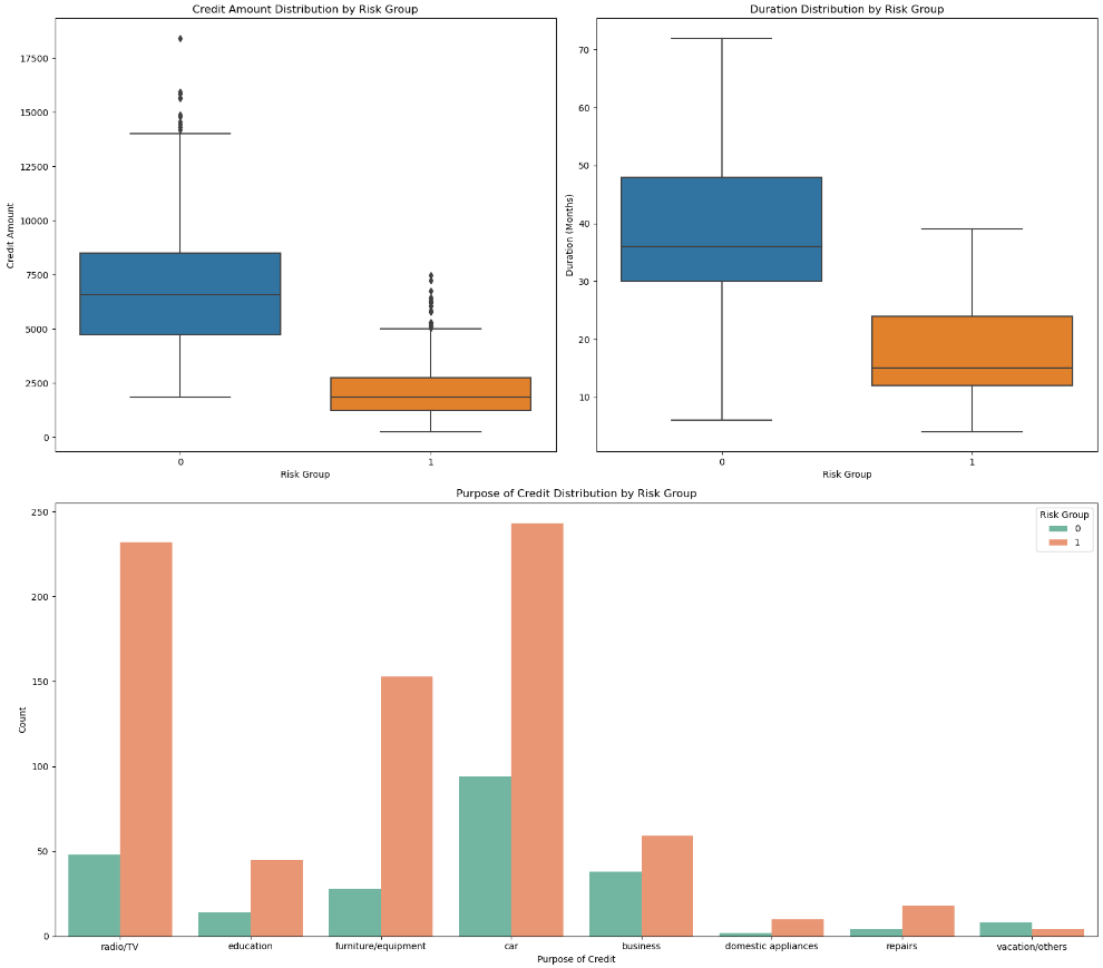
案例3

# 贷款情况对比¶
fig = plt.figure(figsize=(17,15))
 
# 创建2x2的图布局
ax1 = fig.add_subplot(2, 2, 1)
ax2 = fig.add_subplot(2, 2, 2)
ax3 = fig.add_subplot(2, 1, 2)
 
sns.boxplot(x='Risk Group', y='Credit amount', data=data, ax=ax1)
ax1.set_title('Credit Amount Distribution by Risk Group')
ax1.set_xlabel('Risk Group')
ax1.set_ylabel('Credit Amount')
 
sns.boxplot(x='Risk Group', y='Duration', data=data, ax=ax2)
ax2.set_title('Duration Distribution by Risk Group')
ax2.set_xlabel('Risk Group')
ax2.set_ylabel('Duration (Months)')
 
sns.countplot(x='Purpose', hue='Risk Group', data=data, palette='Set2', ax=ax3)
ax3.set_title('Purpose of Credit Distribution by Risk Group')
ax3.set_xlabel('Purpose of Credit')
ax3.set_ylabel('Count')
 
plt.tight_layout()
plt.show()

查看详情

• 输出
  

• 结论

通过三类不同情况的分析，可以初步判断，0为高风险人群，1为低风险人群，原因如下：
1.类型1不仅借款金额远小于类型0，并且借款周期也远小于类型0，表明类型0的客户还款负担更重。
2.类型0虽然资金更加充足(储蓄账户状况、支票账户状况)，但是通过贷款用途可以看到，主要用于商业和购买车子(占比更大)，可以初步判断类型1中，有一些商人，从职业等级也能看出来，大部分在2和3，这一类人群，虽然有钱，但是开销也大，因此风险比类型1高。
因此，可以认为类型1属于低风险用户，类型0属于高风险用户，因为没有违约数据，这里只能通过聚类来简单划分一下。

案例4

# 用户画像分析
# 这步与上一步不同，我这里并没有将风险评估的情况放到聚类数据中，这样可以通过原始数据更好的确定聚类数与聚类情况，并且可以根据聚类结果判断风险评估是否准确。
 
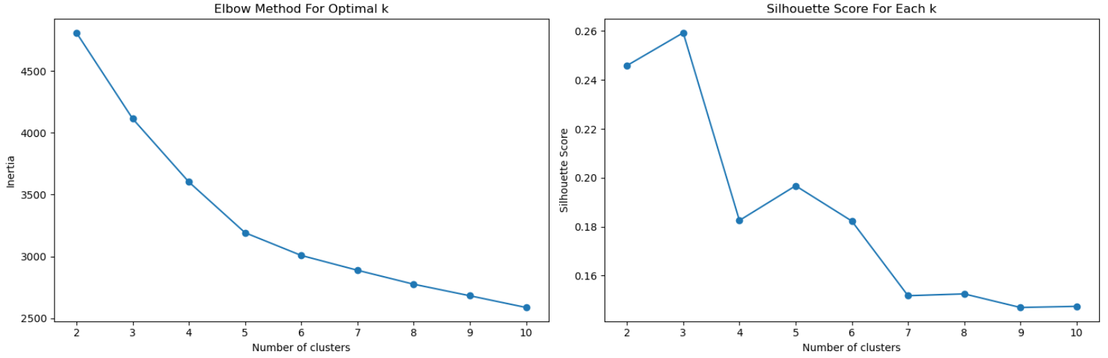
# 使用肘部法则来确定最佳聚类数
inertia = []
silhouette_scores = []
k_range = range(2, 11)
for k in k_range:
    kmeans = KMeans(n_clusters=k, random_state=10).fit(new_data)
    inertia.append(kmeans.inertia_)
    silhouette_scores.append(silhouette_score(new_data, kmeans.labels_))
plt.figure(figsize=(15,5))
 
plt.subplot(1, 2, 1)
plt.plot(k_range, inertia, marker='o')
plt.xlabel('Number of clusters')
plt.ylabel('Inertia')
plt.title('Elbow Method For Optimal k')
 
plt.subplot(1, 2, 2)
plt.plot(k_range, silhouette_scores, marker='o')
plt.xlabel('Number of clusters')
plt.ylabel('Silhouette Score')
plt.title('Silhouette Score For Each k')
 
plt.tight_layout()
plt.show()

查看详情

• 输出
  

• 结论

1.左图为肘部法则图，通过此图可以看到，在4和5的时候，曲线下降速率明显下降。
2.右图为轮廓系数图，在2时，轮廓系数最高，在4时也不错。
结合两个图，我们选择4作为聚类数，此时肘部法则图下降速率有明显下降，且是轮廓系数图中第二高的点。

案例5

# 建立k均值聚类模型
# 执行K-均值聚类，选择4个聚类
kmeans_final = KMeans(n_clusters=4, random_state=15)
kmeans_final.fit(new_data)
# 获取聚类标签
cluster_labels = kmeans_final.labels_
# 将聚类标签添加到原始数据中以进行分析
data['Cluster'] = cluster_labels
 
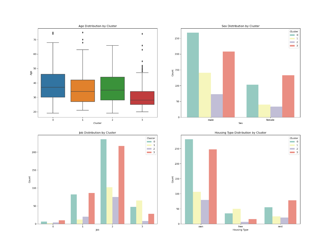
# 四类客户之间对比
# 基本情况对比
fig, axs = plt.subplots(2, 2, figsize=(20,15))
 
sns.boxplot(x='Cluster', y='Age', data=data, ax=axs[0, 0])
axs[0, 0].set_title('Age Distribution by Cluster')
axs[0, 0].set_xlabel('Cluster')
axs[0, 0].set_ylabel('Age')
 
sns.countplot(x='Sex', hue='Cluster', data=data, palette='Set3', ax=axs[0, 1])
axs[0, 1].set_title('Sex Distribution by Cluster')
axs[0, 1].set_xlabel('Sex')
axs[0, 1].set_ylabel('Count')
 
sns.countplot(x='Job', hue='Cluster', data=data, palette='Set3', ax=axs[1, 0])
axs[1, 0].set_title('Job Distribution by Cluster')
axs[1, 0].set_xlabel('Job')
axs[1, 0].set_ylabel('Count')
 
sns.countplot(x='Housing', hue='Cluster', data=data, palette='Set3', ax=axs[1, 1])
axs[1, 1].set_title('Housing Type Distribution by Cluster')
axs[1, 1].set_xlabel('Housing Type')
axs[1, 1].set_ylabel('Count')
plt.show()

查看详情

• 输出
  

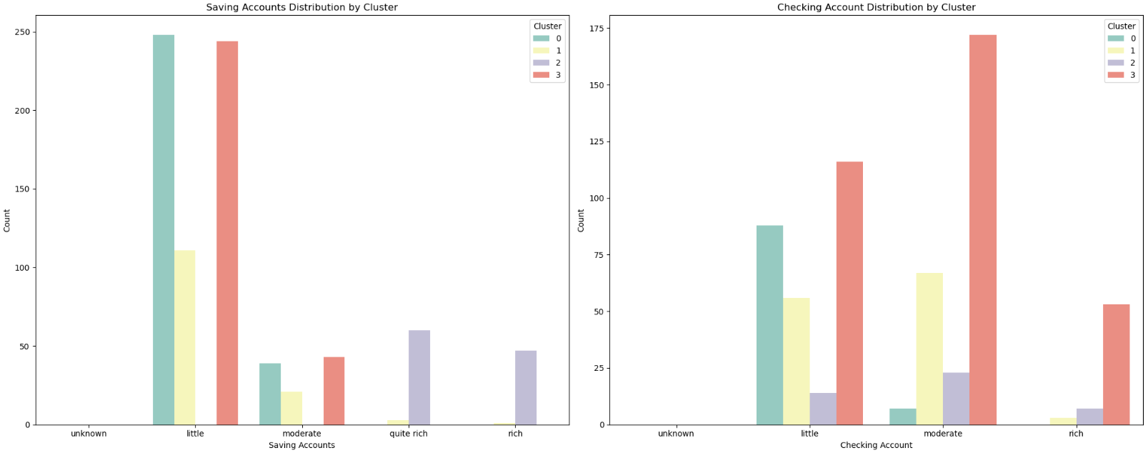
案例6

# 经济情况对比
order_savings = ['unknown', 'little', 'moderate', 'quite rich', 'rich']
order_checking = ['unknown', 'little', 'moderate', 'rich']
 
fig, axs = plt.subplots(1, 2, figsize=(20,8))
 
sns.countplot(x='Saving accounts', hue='Cluster', data=data, order=order_savings, palette='Set3', ax=axs[0])
axs[0].set_title('Saving Accounts Distribution by Cluster')
axs[0].set_xlabel('Saving Accounts')
axs[0].set_ylabel('Count')
axs[0].legend(title='Cluster', loc='upper right')
 
sns.countplot(x='Checking account', hue='Cluster', data=data, order=order_checking, palette='Set3', ax=axs[1])
axs[1].set_title('Checking Account Distribution by Cluster')
axs[1].set_xlabel('Checking Account')
axs[1].set_ylabel('Count')
 
plt.tight_layout()
plt.show()

查看详情

• 输出
  

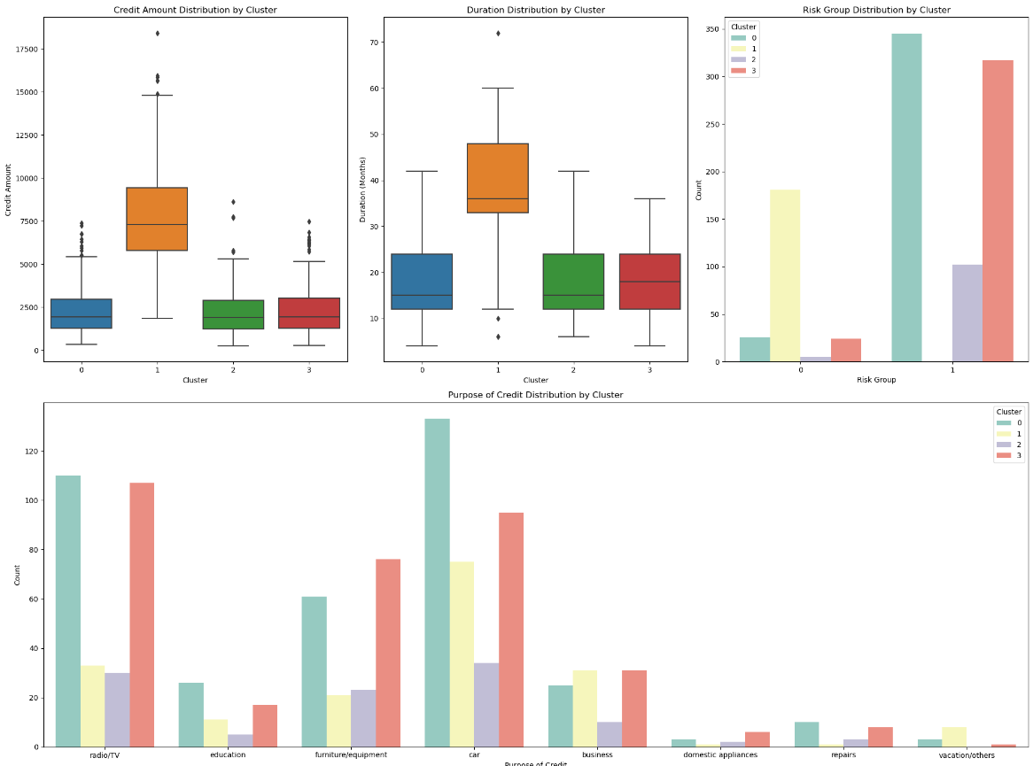
案例7

# 贷款情况对比
fig = plt.figure(figsize=(20,15))
 
# 创建2x2的图布局
ax1 = fig.add_subplot(2, 3, 1)
ax2 = fig.add_subplot(2, 3, 2)
ax3 = fig.add_subplot(2, 3, 3)
ax4 = fig.add_subplot(2, 1, 2)
 
sns.boxplot(x='Cluster', y='Credit amount', data=data, ax=ax1)
ax1.set_title('Credit Amount Distribution by Cluster')
ax1.set_xlabel('Cluster')
ax1.set_ylabel('Credit Amount')
 
sns.boxplot(x='Cluster', y='Duration', data=data, ax=ax2)
ax2.set_title('Duration Distribution by Cluster')
ax2.set_xlabel('Cluster')
ax2.set_ylabel('Duration (Months)')
 
sns.countplot(x='Risk Group', hue='Cluster', data=data, palette='Set3', ax=ax3)
ax3.set_title('Risk Group Distribution by Cluster')
ax3.set_xlabel('Risk Group')
ax3.set_ylabel('Count')
 
sns.countplot(x='Purpose', hue='Cluster', data=data, palette='Set3', ax=ax4)
ax4.set_title('Purpose of Credit Distribution by Cluster')
ax4.set_xlabel('Purpose of Credit')
ax4.set_ylabel('Count')
 
plt.tight_layout()
plt.show()

查看详情

• 输出
  

• 结论

1.类型0（中高等额度需求，倾向于中长期贷款的高职业人群）:
用户画像：年龄主要在20-40岁之间，职业主要在2-3级，这一类人是住免租赁或者租房的占比远高于其他三类，储蓄账户状况主要集中在未知和少量，支票账户也是如此，主要集中在未知、少量和适中，贷款金额和贷款周期远超其他三类，贷款主要用于购车，根据风险评估，这类客户全部为高风险。
建议：银行和金融机构可以为这个群体提供中期汽车贷款产品，并且可以通过金融教育来提升他们的储蓄和投资能力。
2.类别1（较高储蓄能力，倾向于短期贷款的人群）:
用户画像：年龄分布比较均匀，与类型0相近，职业主要在2级，免租赁的占比较小，储蓄账户状况远超其他三类客户，贷款金额少，周期短，贷款主要用于购买设备，根据风险评估，这类客户全部为低风险。
建议：银行和金融机构可以为这个群体提供短期信用产品，同时考虑他们较高的储蓄能力，可以推广储蓄和投资相关产品。
3.类型2（短期贷款，储蓄能力有限的年轻化人群）:
用户画像：平均年龄在30岁以下，最大年龄不超过45岁，比其他三类都更年轻，职业主要集中在2级，但是其他等级都有存在，租房占比高于其他三类，蓄账户状况主要集中在未知和少量，支票账户主要集中在未知、少量和适中，这类客户的资金情况与类型0类似，贷款情况与类型1类似，风险评估绝大多数为低风险。
建议：鉴于他们是信用初建者和年轻消费者，银行和金融机构可以提供小额信用卡产品和财务规划服务。
4.类型3（短期贷款的高龄客户）:
用户画像：大龄客户，职业集中在1-2级，大部分有自己的房子，少部分是免租赁，蓄账户状况主要集中在未知和少量，支票账户每个等级均有占比，贷款情况与类型1和类型2类似，也是贷款金额少，周期短，同样的风险评估大多数是低风险。
建议：针对这类客户，银行和金融机构可以提供针对成熟消费者的产品和服务，如退休规划和健康保险，同时关注其稳定的信贷需求。