week_15_Random_Forest
霉霉数据分析——基于pandas库
背景


摘录《Taylor Swift The Whole Story》


目的
我们尝试通过taylor swift的数据集分析人气单曲、具有舞蹈性和活力的单曲、各个特征的相关程度、专辑流行度。
变量描述
popularity:流行度
Danceability: 舞蹈性
Acousticness: 原声,值越高,歌曲的原声性越强对应为不插电
Energy: 歌曲的能量
instrumentalness:乐器表现
liveness:现场感
Loudness: 响度,值越高,歌曲越响亮
Speechiness: 口语化,值越高,歌词越口语化
Valence: 效价(情绪),值越高,这首歌的情绪就越积极正能量
tempo:节奏感
读入数据
import numpy as np # linear algebra
import pandas as pd # data processing, CSV file I/O (e.g. pd.read_csv)
tay = pd.read_csv('spotify_taylorswift.csv')
tay.head()
| Unnamed: 0 | name | album | artist | release_date | length | popularity | danceability | acousticness | energy | instrumentalness | liveness | loudness | speechiness | valence | tempo | |
|---|---|---|---|---|---|---|---|---|---|---|---|---|---|---|---|---|
| 0 | 0 | Tim McGraw | Taylor Swift | Taylor Swift | 2006-10-24 | 232106 | 49 | 0.580 | 0.575 | 0.491 | 0.0 | 0.1210 | -6.462 | 0.0251 | 0.425 | 76.009 |
| 1 | 1 | Picture To Burn | Taylor Swift | Taylor Swift | 2006-10-24 | 173066 | 54 | 0.658 | 0.173 | 0.877 | 0.0 | 0.0962 | -2.098 | 0.0323 | 0.821 | 105.586 |
| 2 | 2 | Teardrops On My Guitar - Radio Single Remix | Taylor Swift | Taylor Swift | 2006-10-24 | 203040 | 59 | 0.621 | 0.288 | 0.417 | 0.0 | 0.1190 | -6.941 | 0.0231 | 0.289 | 99.953 |
| 3 | 3 | A Place in this World | Taylor Swift | Taylor Swift | 2006-10-24 | 199200 | 49 | 0.576 | 0.051 | 0.777 | 0.0 | 0.3200 | -2.881 | 0.0324 | 0.428 | 115.028 |
| 4 | 4 | Cold As You | Taylor Swift | Taylor Swift | 2006-10-24 | 239013 | 50 | 0.418 | 0.217 | 0.482 | 0.0 | 0.1230 | -5.769 | 0.0266 | 0.261 | 175.558 |
数据预处理
删除第一列索引
del tay[tay.keys()[0]]
tay.head()
| name | album | artist | release_date | length | popularity | danceability | acousticness | energy | instrumentalness | liveness | loudness | speechiness | valence | tempo | |
|---|---|---|---|---|---|---|---|---|---|---|---|---|---|---|---|
| 0 | Tim McGraw | Taylor Swift | Taylor Swift | 2006-10-24 | 232106 | 49 | 0.580 | 0.575 | 0.491 | 0.0 | 0.1210 | -6.462 | 0.0251 | 0.425 | 76.009 |
| 1 | Picture To Burn | Taylor Swift | Taylor Swift | 2006-10-24 | 173066 | 54 | 0.658 | 0.173 | 0.877 | 0.0 | 0.0962 | -2.098 | 0.0323 | 0.821 | 105.586 |
| 2 | Teardrops On My Guitar - Radio Single Remix | Taylor Swift | Taylor Swift | 2006-10-24 | 203040 | 59 | 0.621 | 0.288 | 0.417 | 0.0 | 0.1190 | -6.941 | 0.0231 | 0.289 | 99.953 |
| 3 | A Place in this World | Taylor Swift | Taylor Swift | 2006-10-24 | 199200 | 49 | 0.576 | 0.051 | 0.777 | 0.0 | 0.3200 | -2.881 | 0.0324 | 0.428 | 115.028 |
| 4 | Cold As You | Taylor Swift | Taylor Swift | 2006-10-24 | 239013 | 50 | 0.418 | 0.217 | 0.482 | 0.0 | 0.1230 | -5.769 | 0.0266 | 0.261 | 175.558 |
删除空值的样本
tay.info()
<class 'pandas.core.frame.DataFrame'>
RangeIndex: 171 entries, 0 to 170
Data columns (total 15 columns):
 #   Column            Non-Null Count  Dtype
---  ------            --------------  -----
 0   name              171 non-null    object
 1   album             171 non-null    object
 2   artist            171 non-null    object
 3   release_date      171 non-null    object
 4   length            171 non-null    int64
 5   popularity        171 non-null    int64
 6   danceability      171 non-null    float64
 7   acousticness      171 non-null    float64
 8   energy            171 non-null    float64
 9   instrumentalness  171 non-null    float64
 10  liveness          171 non-null    float64
 11  loudness          171 non-null    float64
 12  speechiness       171 non-null    float64
 13  valence           171 non-null    float64
 14  tempo             171 non-null    float64
dtypes: float64(9), int64(2), object(4)
memory usage: 20.2+ KB
tay = tay.dropna()
tay.info()
<class 'pandas.core.frame.DataFrame'>
RangeIndex: 171 entries, 0 to 170
Data columns (total 15 columns):
 #   Column            Non-Null Count  Dtype
---  ------            --------------  -----
 0   name              171 non-null    object
 1   album             171 non-null    object
 2   artist            171 non-null    object
 3   release_date      171 non-null    object
 4   length            171 non-null    int64
 5   popularity        171 non-null    int64
 6   danceability      171 non-null    float64
 7   acousticness      171 non-null    float64
 8   energy            171 non-null    float64
 9   instrumentalness  171 non-null    float64
 10  liveness          171 non-null    float64
 11  loudness          171 non-null    float64
 12  speechiness       171 non-null    float64
 13  valence           171 non-null    float64
 14  tempo             171 non-null    float64
dtypes: float64(9), int64(2), object(4)
memory usage: 20.2+ KB
人气排序
#用sort_values对人气进行排序,以获得泰勒最受欢迎的歌曲。
populars = tay.sort_values(by='popularity', ascending=False)

populars.head(13)
| name | album | artist | release_date | length | popularity | danceability | acousticness | energy | instrumentalness | liveness | loudness | speechiness | valence | tempo | |
|---|---|---|---|---|---|---|---|---|---|---|---|---|---|---|---|
| 60 | Blank Space | 1989 (Deluxe) | Taylor Swift | 2014-01-01 | 231826 | 82 | 0.760 | 0.10300 | 0.703 | 0.000000 | 0.0913 | -5.412 | 0.0540 | 0.5700 | 95.997 |
| 64 | Shake It Off | 1989 (Deluxe) | Taylor Swift | 2014-01-01 | 219200 | 80 | 0.647 | 0.06470 | 0.800 | 0.000000 | 0.3340 | -5.384 | 0.1650 | 0.9420 | 160.078 |
| 95 | Lover | Lover | Taylor Swift | 2019-08-23 | 221306 | 80 | 0.359 | 0.49200 | 0.543 | 0.000016 | 0.1180 | -7.582 | 0.0919 | 0.4530 | 68.534 |
| 82 | Delicate | reputation | Taylor Swift | 2017-11-10 | 232253 | 78 | 0.750 | 0.21600 | 0.404 | 0.000357 | 0.0911 | -10.178 | 0.0682 | 0.0499 | 95.045 |
| 106 | You Need To Calm Down | Lover | Taylor Swift | 2019-08-23 | 171360 | 78 | 0.771 | 0.00929 | 0.671 | 0.000000 | 0.0637 | -5.617 | 0.0553 | 0.7140 | 85.026 |
| 94 | Cruel Summer | Lover | Taylor Swift | 2019-08-23 | 178426 | 77 | 0.552 | 0.11700 | 0.702 | 0.000021 | 0.1050 | -5.707 | 0.1570 | 0.5640 | 169.994 |
| 108 | ME! (feat. Brendon Urie of Panic! At The Disco) | Lover | Taylor Swift | 2019-08-23 | 193000 | 77 | 0.610 | 0.03300 | 0.830 | 0.000000 | 0.1180 | -4.105 | 0.0571 | 0.7280 | 182.162 |
| 83 | Look What You Made Me Do | reputation | Taylor Swift | 2017-11-10 | 211853 | 77 | 0.766 | 0.20400 | 0.709 | 0.000014 | 0.1260 | -6.471 | 0.1230 | 0.5060 | 128.070 |
| 86 | Getaway Car | reputation | Taylor Swift | 2017-11-10 | 233626 | 76 | 0.562 | 0.00465 | 0.689 | 0.000002 | 0.0888 | -6.745 | 0.1270 | 0.3510 | 172.054 |
| 150 | You Belong With Me (Taylor’s Version) | Fearless (Taylor's Version) | Taylor Swift | 2021-04-09 | 231124 | 76 | 0.632 | 0.06230 | 0.773 | 0.000000 | 0.0885 | -4.856 | 0.0346 | 0.4740 | 130.033 |
| 100 | Paper Rings | Lover | Taylor Swift | 2019-08-23 | 222400 | 76 | 0.811 | 0.01290 | 0.719 | 0.000014 | 0.0742 | -6.553 | 0.0497 | 0.8650 | 103.979 |
| 81 | Don’t Blame Me | reputation | Taylor Swift | 2017-11-10 | 236413 | 75 | 0.615 | 0.10600 | 0.534 | 0.000018 | 0.0607 | -6.719 | 0.0386 | 0.1930 | 135.917 |
| 61 | Style | 1989 (Deluxe) | Taylor Swift | 2014-01-01 | 231000 | 75 | 0.588 | 0.00245 | 0.791 | 0.002580 | 0.1180 | -5.595 | 0.0402 | 0.4870 | 94.933 |
提取 TOP 5 单曲
top_5 = populars.head()

#loc是用来访问一组行和列
top_5.loc[:,['name','popularity']]
| name | popularity | |
|---|---|---|
| 60 | Blank Space | 82 |
| 64 | Shake It Off | 80 |
| 95 | Lover | 80 |
| 82 | Delicate | 78 |
| 106 | You Need To Calm Down | 78 |
提取舞蹈性较高的单曲
#有一栏danceability - 舞蹈性,我们要过滤掉那些舞蹈性最高的歌曲(即,超过0.75)。
dance_on = tay.loc[(tay.danceability >= 0.75)]
dance_on.loc[:,['name','album','danceability']].head(13)
| name | album | danceability | |
|---|---|---|---|
| 56 | Treacherous - Original Demo Recording | Red (Deluxe Edition) | 0.828 |
| 59 | Welcome To New York | 1989 (Deluxe) | 0.789 |
| 60 | Blank Space | 1989 (Deluxe) | 0.760 |
| 68 | How You Get The Girl | 1989 (Deluxe) | 0.765 |
| 71 | Clean | 1989 (Deluxe) | 0.815 |
| 76 | I Wish You Would - Voice Memo | 1989 (Deluxe) | 0.781 |
| 82 | Delicate | reputation | 0.750 |
| 83 | Look What You Made Me Do | reputation | 0.766 |
| 85 | Gorgeous | reputation | 0.800 |
| 96 | The Man | Lover | 0.777 |
| 98 | I Think He Knows | Lover | 0.897 |
| 100 | Paper Rings | Lover | 0.811 |
| 101 | Cornelia Street | Lover | 0.824 |
提取活力值较高的单曲
energy = tay.loc[(tay.energy >= 0.5)]

energy = tay.sort_values(by='energy', ascending=False)

energy.loc[:,['name','album','energy']].head(13)
| name | album | energy | |
|---|---|---|---|
| 26 | Haunted | Speak Now (Deluxe Package) | 0.944 |
| 11 | I'm Only Me When I'm With You | Taylor Swift | 0.934 |
| 24 | Better Than Revenge | Speak Now (Deluxe Package) | 0.917 |
| 152 | Tell Me Why (Taylor’s Version) | Fearless (Taylor's Version) | 0.909 |
| 57 | Red - Original Demo Recording | Red (Deluxe Edition) | 0.902 |
| 38 | Red | Red (Deluxe Edition) | 0.896 |
| 65 | I Wish You Would | 1989 (Deluxe) | 0.893 |
| 74 | New Romantics | 1989 (Deluxe) | 0.889 |
| 1 | Picture To Burn | Taylor Swift | 0.877 |
| 163 | The Other Side Of The Door (Taylor’s Version) | Fearless (Taylor's Version) | 0.873 |
| 21 | The Story Of Us | Speak Now (Deluxe Package) | 0.855 |
| 62 | Out Of The Woods | 1989 (Deluxe) | 0.841 |
| 108 | ME! (feat. Brendon Urie of Panic! At The Disco) | Lover | 0.830 |
查询你最喜欢的专辑
比如,我喜欢《Speak Now》 😃
tay.loc[tay.album == 'Speak Now (Deluxe Package)']
| name | album | artist | release_date | length | popularity | danceability | acousticness | energy | instrumentalness | liveness | loudness | speechiness | valence | tempo | |
|---|---|---|---|---|---|---|---|---|---|---|---|---|---|---|---|
| 15 | Mine - POP Mix | Speak Now (Deluxe Package) | Taylor Swift | 2010-01-01 | 230546 | 45 | 0.696 | 0.004610 | 0.768 | 0.000001 | 0.1010 | -3.863 | 0.0308 | 0.692 | 121.050 |
| 16 | Sparks Fly | Speak Now (Deluxe Package) | Taylor Swift | 2010-01-01 | 260946 | 50 | 0.608 | 0.038700 | 0.785 | 0.000000 | 0.1580 | -2.976 | 0.0311 | 0.376 | 114.985 |
| 17 | Back To December | Speak Now (Deluxe Package) | Taylor Swift | 2010-01-01 | 293040 | 50 | 0.517 | 0.020200 | 0.606 | 0.000000 | 0.3240 | -5.797 | 0.0289 | 0.296 | 141.929 |
| 18 | Speak Now | Speak Now (Deluxe Package) | Taylor Swift | 2010-01-01 | 240773 | 49 | 0.708 | 0.101000 | 0.601 | 0.000000 | 0.0979 | -3.750 | 0.0306 | 0.742 | 118.962 |
| 19 | Dear John | Speak Now (Deluxe Package) | Taylor Swift | 2010-01-01 | 403887 | 48 | 0.583 | 0.183000 | 0.468 | 0.000002 | 0.1110 | -5.378 | 0.0278 | 0.126 | 119.375 |
| 20 | Mean | Speak Now (Deluxe Package) | Taylor Swift | 2010-01-01 | 237746 | 48 | 0.570 | 0.445000 | 0.747 | 0.000000 | 0.2190 | -3.978 | 0.0426 | 0.808 | 164.004 |
| 21 | The Story Of Us | Speak Now (Deluxe Package) | Taylor Swift | 2010-01-01 | 265636 | 48 | 0.575 | 0.000315 | 0.855 | 0.001610 | 0.0419 | -4.827 | 0.0467 | 0.840 | 139.920 |
| 22 | Never Grow Up | Speak Now (Deluxe Package) | Taylor Swift | 2010-01-01 | 290480 | 44 | 0.715 | 0.829000 | 0.308 | 0.000000 | 0.1600 | -8.829 | 0.0305 | 0.547 | 124.899 |
| 23 | Enchanted | Speak Now (Deluxe Package) | Taylor Swift | 2010-01-01 | 352200 | 51 | 0.535 | 0.071600 | 0.618 | 0.000388 | 0.1690 | -3.913 | 0.0273 | 0.228 | 81.975 |
| 24 | Better Than Revenge | Speak Now (Deluxe Package) | Taylor Swift | 2010-01-01 | 217173 | 49 | 0.519 | 0.016700 | 0.917 | 0.000021 | 0.3590 | -3.185 | 0.0887 | 0.652 | 145.882 |
| 25 | Innocent | Speak Now (Deluxe Package) | Taylor Swift | 2010-01-01 | 302266 | 44 | 0.553 | 0.202000 | 0.604 | 0.000000 | 0.1250 | -5.295 | 0.0258 | 0.186 | 133.989 |
| 26 | Haunted | Speak Now (Deluxe Package) | Taylor Swift | 2010-01-01 | 242093 | 47 | 0.434 | 0.076900 | 0.944 | 0.000000 | 0.1510 | -2.641 | 0.0581 | 0.361 | 162.020 |
| 27 | Last Kiss | Speak Now (Deluxe Package) | Taylor Swift | 2010-01-01 | 367146 | 47 | 0.359 | 0.581000 | 0.329 | 0.000037 | 0.0979 | -9.531 | 0.0293 | 0.208 | 84.358 |
| 28 | Long Live | Speak Now (Deluxe Package) | Taylor Swift | 2010-01-01 | 317960 | 47 | 0.412 | 0.042600 | 0.682 | 0.000075 | 0.1060 | -4.319 | 0.0339 | 0.146 | 203.959 |
| 29 | Ours | Speak Now (Deluxe Package) | Taylor Swift | 2010-01-01 | 238173 | 55 | 0.610 | 0.505000 | 0.556 | 0.000000 | 0.0851 | -7.369 | 0.0285 | 0.192 | 159.838 |
| 30 | If This Was A Movie | Speak Now (Deluxe Package) | Taylor Swift | 2010-01-01 | 234546 | 52 | 0.515 | 0.154000 | 0.724 | 0.000004 | 0.2690 | -3.498 | 0.0267 | 0.257 | 147.788 |
| 31 | Superman | Speak Now (Deluxe Package) | Taylor Swift | 2010-01-01 | 276266 | 47 | 0.582 | 0.018700 | 0.817 | 0.000002 | 0.1010 | -3.718 | 0.0337 | 0.547 | 131.983 |
| 32 | Back To December - Acoustic | Speak Now (Deluxe Package) | Taylor Swift | 2010-01-01 | 292533 | 59 | 0.541 | 0.731000 | 0.451 | 0.000000 | 0.1970 | -6.522 | 0.0270 | 0.333 | 141.713 |
| 33 | Haunted - Acoustic Version | Speak Now (Deluxe Package) | Taylor Swift | 2010-01-01 | 217626 | 48 | 0.574 | 0.841000 | 0.462 | 0.000000 | 0.2800 | -5.124 | 0.0252 | 0.314 | 80.858 |
| 34 | Mine | Speak Now (Deluxe Package) | Taylor Swift | 2010-01-01 | 230773 | 64 | 0.621 | 0.003270 | 0.780 | 0.000005 | 0.1840 | -2.934 | 0.0297 | 0.672 | 121.038 |
| 35 | Back To December | Speak Now (Deluxe Package) | Taylor Swift | 2010-01-01 | 293040 | 43 | 0.525 | 0.113000 | 0.676 | 0.000000 | 0.2940 | -4.684 | 0.0294 | 0.281 | 141.950 |
| 36 | The Story Of Us | Speak Now (Deluxe Package) | Taylor Swift | 2010-01-01 | 266480 | 59 | 0.546 | 0.004870 | 0.809 | 0.000372 | 0.0437 | -3.621 | 0.0410 | 0.649 | 139.910 |
分析
查看专辑流行度
#"Taylor Swift","Fearless","Speak Now","Red","1989","Reputation","Lover","Folklore","Evermore"
#59,76,64,72,82,78,80,65,72
#'lightblue','gold','purple','red','tan','black','pink','grey','brown'

album = ["Taylor Swift","Fearless","Speak Now","Red","1989","Reputation","Lover","Folklore","Evermore"]
maxpopularity = [59,76,64,72,82,78,80,65,72]
newcolors = ['lightblue','gold','purple','red','tan','black','pink','grey','brown']

plt.figure( figsize = (8,6))
plt.bar(album, maxpopularity,color = newcolors)
plt.title(' Popularity of albums')
plt.xlabel('ALBUM')
plt.ylabel('POPULARITY')
plt.xticks(fontsize=6)
plt.show()

流行度直方图
sns.displot(x='popularity', data=tay, kde=True, color='#a70ad5')
plt.title('Popularity Distribution')
Text(0.5, 1.0, 'Popularity Distribution')

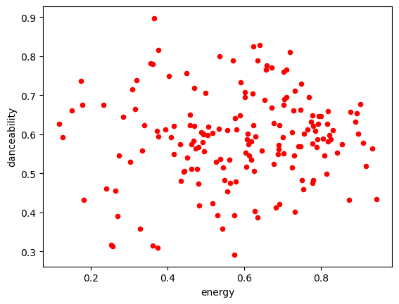
以活力值和舞蹈性为例
import matplotlib.pyplot as plt
import numpy as np
energyy = tay.energy
dancee = tay.danceability

correlation_length = energyy.corr(dancee)
print(correlation_length)
ax1 = tay.plot.scatter(x = 'energy',y = 'danceability',c = 'red')
0.06266927386034048
Energy 和 Acousticness的相关性
sns.set_theme(color_codes=True)
plt.figure(figsize=(18, 6))
sns.regplot(x='acousticness', y='energy', data=tay)
plt.title('Acousticness vs Energy')
Text(0.5, 1.0, 'Acousticness vs Energy')

Energy 和 Loudness相关性
sns.set_theme(color_codes=True)
plt.figure(figsize=(18, 6))
sns.regplot(x='energy', y='loudness', data=tay)
plt.title('Energy vs Loudness')
Text(0.5, 1.0, 'Energy vs Loudness')

相关系数矩阵
tay.corr()
C:\Users\dogfa\AppData\Local\Temp\ipykernel_10964\3121711199.py:1: FutureWarning: The default value of numeric_only in DataFrame.corr is deprecated. In a future version, it will default to False. Select only valid columns or specify the value of numeric_only to silence this warning.
  tay.corr()
| length | popularity | danceability | acousticness | energy | instrumentalness | liveness | loudness | speechiness | valence | tempo | |
|---|---|---|---|---|---|---|---|---|---|---|---|
| length | 1.000000 | 0.011772 | -0.301561 | 0.038749 | -0.114792 | -0.081288 | -0.148412 | 0.044126 | -0.414447 | -0.420405 | 0.010425 |
| popularity | 0.011772 | 1.000000 | 0.072622 | -0.117842 | 0.127495 | 0.035638 | -0.406730 | 0.122576 | -0.478262 | 0.034154 | -0.015669 |
| danceability | -0.301561 | 0.072622 | 1.000000 | -0.143085 | 0.062669 | -0.051837 | -0.015766 | 0.002587 | 0.183860 | 0.379786 | -0.235370 |
| acousticness | 0.038749 | -0.117842 | -0.143085 | 1.000000 | -0.710055 | 0.140655 | -0.065387 | -0.736624 | 0.143127 | -0.231232 | -0.134467 |
| energy | -0.114792 | 0.127495 | 0.062669 | -0.710055 | 1.000000 | 0.000281 | 0.046364 | 0.784973 | -0.179336 | 0.490371 | 0.209914 |
| instrumentalness | -0.081288 | 0.035638 | -0.051837 | 0.140655 | 0.000281 | 1.000000 | -0.059132 | -0.084224 | -0.029729 | 0.020076 | 0.043274 |
| liveness | -0.148412 | -0.406730 | -0.015766 | -0.065387 | 0.046364 | -0.059132 | 1.000000 | 0.016324 | 0.357924 | -0.017264 | 0.034934 |
| loudness | 0.044126 | 0.122576 | 0.002587 | -0.736624 | 0.784973 | -0.084224 | 0.016324 | 1.000000 | -0.409577 | 0.299926 | 0.171503 |
| speechiness | -0.414447 | -0.478262 | 0.183860 | 0.143127 | -0.179336 | -0.029729 | 0.357924 | -0.409577 | 1.000000 | 0.120352 | -0.027812 |
| valence | -0.420405 | 0.034154 | 0.379786 | -0.231232 | 0.490371 | 0.020076 | -0.017264 | 0.299926 | 0.120352 | 1.000000 | -0.006056 |
| tempo | 0.010425 | -0.015669 | -0.235370 | -0.134467 | 0.209914 | 0.043274 | 0.034934 | 0.171503 | -0.027812 | -0.006056 | 1.000000 |
相关系数矩阵图
import seaborn as sns
import matplotlib.pyplot as plt
sns.heatmap(tay.corr())
C:\Users\dogfa\AppData\Local\Temp\ipykernel_10964\54934055.py:1: FutureWarning: The default value of numeric_only in DataFrame.corr is deprecated. In a future version, it will default to False. Select only valid columns or specify the value of numeric_only to silence this warning.
  sns.heatmap(tay.corr())


<Axes: >

相关性矩阵图
sns.pairplot(tay[2:])
<seaborn.axisgrid.PairGrid at 0x29d8b437b50>

Random Forest Regression
算法原理
随机森林中的每棵树在称为自助聚集 (bagging) 的过程中随机对训练数据子集进行抽样。该模型适合这些较小的数据集,并汇总预测结果。通过有放回抽样,可以重复使用同一数据的几个实例,结果就是,这些树不仅基于不同的数据集进行训练,而且还使用不同的特性做出决策。

整理数据
# 删除album列
dataset = tay.drop(['album','artist','release_date','name'], axis=1)

dataset
| length | popularity | danceability | acousticness | energy | instrumentalness | liveness | loudness | speechiness | valence | tempo | |
|---|---|---|---|---|---|---|---|---|---|---|---|
| 0 | 232106 | 49 | 0.580 | 0.575 | 0.491 | 0.000000 | 0.1210 | -6.462 | 0.0251 | 0.425 | 76.009 |
| 1 | 173066 | 54 | 0.658 | 0.173 | 0.877 | 0.000000 | 0.0962 | -2.098 | 0.0323 | 0.821 | 105.586 |
| 2 | 203040 | 59 | 0.621 | 0.288 | 0.417 | 0.000000 | 0.1190 | -6.941 | 0.0231 | 0.289 | 99.953 |
| 3 | 199200 | 49 | 0.576 | 0.051 | 0.777 | 0.000000 | 0.3200 | -2.881 | 0.0324 | 0.428 | 115.028 |
| 4 | 239013 | 50 | 0.418 | 0.217 | 0.482 | 0.000000 | 0.1230 | -5.769 | 0.0266 | 0.261 | 175.558 |
| ... | ... | ... | ... | ... | ... | ... | ... | ... | ... | ... | ... |
| 166 | 277591 | 74 | 0.660 | 0.162 | 0.817 | 0.000000 | 0.0667 | -6.269 | 0.0521 | 0.714 | 135.942 |
| 167 | 244236 | 65 | 0.609 | 0.849 | 0.373 | 0.000000 | 0.0779 | -8.819 | 0.0263 | 0.130 | 106.007 |
| 168 | 189495 | 67 | 0.588 | 0.225 | 0.608 | 0.000000 | 0.0920 | -7.062 | 0.0365 | 0.508 | 90.201 |
| 169 | 208608 | 66 | 0.563 | 0.514 | 0.473 | 0.000012 | 0.1090 | -11.548 | 0.0503 | 0.405 | 101.934 |
| 170 | 242157 | 64 | 0.624 | 0.334 | 0.624 | 0.000000 | 0.0995 | -7.860 | 0.0539 | 0.527 | 80.132 |
171 rows × 11 columns
x = dataset.drop(['popularity'],axis=1)
x
| length | danceability | acousticness | energy | instrumentalness | liveness | loudness | speechiness | valence | tempo | |
|---|---|---|---|---|---|---|---|---|---|---|
| 0 | 232106 | 0.580 | 0.575 | 0.491 | 0.000000 | 0.1210 | -6.462 | 0.0251 | 0.425 | 76.009 |
| 1 | 173066 | 0.658 | 0.173 | 0.877 | 0.000000 | 0.0962 | -2.098 | 0.0323 | 0.821 | 105.586 |
| 2 | 203040 | 0.621 | 0.288 | 0.417 | 0.000000 | 0.1190 | -6.941 | 0.0231 | 0.289 | 99.953 |
| 3 | 199200 | 0.576 | 0.051 | 0.777 | 0.000000 | 0.3200 | -2.881 | 0.0324 | 0.428 | 115.028 |
| 4 | 239013 | 0.418 | 0.217 | 0.482 | 0.000000 | 0.1230 | -5.769 | 0.0266 | 0.261 | 175.558 |
| ... | ... | ... | ... | ... | ... | ... | ... | ... | ... | ... |
| 166 | 277591 | 0.660 | 0.162 | 0.817 | 0.000000 | 0.0667 | -6.269 | 0.0521 | 0.714 | 135.942 |
| 167 | 244236 | 0.609 | 0.849 | 0.373 | 0.000000 | 0.0779 | -8.819 | 0.0263 | 0.130 | 106.007 |
| 168 | 189495 | 0.588 | 0.225 | 0.608 | 0.000000 | 0.0920 | -7.062 | 0.0365 | 0.508 | 90.201 |
| 169 | 208608 | 0.563 | 0.514 | 0.473 | 0.000012 | 0.1090 | -11.548 | 0.0503 | 0.405 | 101.934 |
| 170 | 242157 | 0.624 | 0.334 | 0.624 | 0.000000 | 0.0995 | -7.860 | 0.0539 | 0.527 | 80.132 |
171 rows × 10 columns
y = dataset['popularity']
y
0      49
1      54
2      59
3      49
4      50
       ..
166    74
167    65
168    67
169    66
170    64
Name: popularity, Length: 171, dtype: int64
划分train test
from sklearn.model_selection import train_test_split
x_train, x_test, y_train, y_test = train_test_split(x,y, test_size=0.2,random_state=1)
x_train
| length | danceability | acousticness | energy | instrumentalness | liveness | loudness | speechiness | valence | tempo | |
|---|---|---|---|---|---|---|---|---|---|---|
| 89 | 230373 | 0.719 | 0.032900 | 0.469 | 0.000000 | 0.1690 | -8.792 | 0.0533 | 0.0851 | 120.085 |
| 88 | 211506 | 0.624 | 0.060400 | 0.691 | 0.000011 | 0.1380 | -6.686 | 0.1960 | 0.2840 | 160.024 |
| 165 | 220839 | 0.599 | 0.816000 | 0.494 | 0.000000 | 0.1010 | -7.610 | 0.0372 | 0.4400 | 142.893 |
| 110 | 293453 | 0.557 | 0.808000 | 0.496 | 0.000173 | 0.0772 | -9.602 | 0.0563 | 0.2650 | 149.983 |
| 48 | 284866 | 0.624 | 0.632000 | 0.340 | 0.033700 | 0.0805 | -12.411 | 0.0290 | 0.2610 | 129.987 |
| ... | ... | ... | ... | ... | ... | ... | ... | ... | ... | ... |
| 133 | 215626 | 0.546 | 0.418000 | 0.613 | 0.000000 | 0.1030 | -7.589 | 0.0264 | 0.5350 | 79.015 |
| 137 | 260440 | 0.515 | 0.855000 | 0.545 | 0.000020 | 0.0921 | -9.277 | 0.0353 | 0.5350 | 88.856 |
| 72 | 245560 | 0.422 | 0.049300 | 0.692 | 0.000026 | 0.1770 | -5.447 | 0.0549 | 0.1970 | 184.014 |
| 140 | 257773 | 0.535 | 0.876000 | 0.561 | 0.000136 | 0.1150 | -11.609 | 0.0484 | 0.2870 | 96.103 |
| 37 | 295720 | 0.588 | 0.000197 | 0.825 | 0.001380 | 0.0884 | -5.882 | 0.0328 | 0.3970 | 129.968 |
136 rows × 10 columns
x_test
| length | danceability | acousticness | energy | instrumentalness | liveness | loudness | speechiness | valence | tempo | |
|---|---|---|---|---|---|---|---|---|---|---|
| 92 | 235466 | 0.661 | 0.921000 | 0.151 | 0.000000 | 0.1300 | -12.864 | 0.0354 | 0.230 | 94.922 |
| 113 | 231000 | 0.688 | 0.481000 | 0.653 | 0.004140 | 0.1060 | -8.558 | 0.0403 | 0.701 | 147.991 |
| 19 | 403887 | 0.583 | 0.183000 | 0.468 | 0.000002 | 0.1110 | -5.378 | 0.0278 | 0.126 | 119.375 |
| 69 | 250093 | 0.481 | 0.678000 | 0.435 | 0.000000 | 0.0928 | -8.795 | 0.0321 | 0.107 | 143.950 |
| 53 | 286613 | 0.619 | 0.187000 | 0.506 | 0.000015 | 0.1010 | -7.327 | 0.0315 | 0.274 | 126.030 |
| 161 | 237338 | 0.476 | 0.040600 | 0.564 | 0.000000 | 0.1020 | -5.677 | 0.0269 | 0.167 | 143.929 |
| 108 | 193000 | 0.610 | 0.033000 | 0.830 | 0.000000 | 0.1180 | -4.105 | 0.0571 | 0.728 | 182.162 |
| 14 | 179066 | 0.459 | 0.040200 | 0.753 | 0.000000 | 0.0863 | -3.827 | 0.0537 | 0.483 | 199.997 |
| 99 | 234146 | 0.662 | 0.028000 | 0.747 | 0.006150 | 0.1380 | -6.926 | 0.0736 | 0.487 | 150.088 |
| 107 | 223293 | 0.756 | 0.130000 | 0.449 | 0.000000 | 0.1140 | -8.746 | 0.0344 | 0.399 | 111.011 |
| 11 | 213053 | 0.563 | 0.004520 | 0.934 | 0.000807 | 0.1030 | -3.629 | 0.0646 | 0.518 | 143.964 |
| 4 | 239013 | 0.418 | 0.217000 | 0.482 | 0.000000 | 0.1230 | -5.769 | 0.0266 | 0.261 | 175.558 |
| 117 | 208906 | 0.602 | 0.888000 | 0.494 | 0.000026 | 0.0902 | -10.813 | 0.0277 | 0.374 | 94.955 |
| 42 | 232120 | 0.661 | 0.002150 | 0.729 | 0.001300 | 0.0477 | -6.561 | 0.0376 | 0.668 | 103.987 |
| 122 | 237266 | 0.593 | 0.670000 | 0.700 | 0.000007 | 0.1160 | -9.016 | 0.0492 | 0.451 | 141.898 |
| 125 | 234000 | 0.644 | 0.916000 | 0.284 | 0.000015 | 0.0909 | -12.879 | 0.0821 | 0.328 | 150.072 |
| 147 | 235766 | 0.627 | 0.130000 | 0.792 | 0.000004 | 0.0845 | -4.311 | 0.0310 | 0.415 | 119.054 |
| 35 | 293040 | 0.525 | 0.113000 | 0.676 | 0.000000 | 0.2940 | -4.684 | 0.0294 | 0.281 | 141.950 |
| 81 | 236413 | 0.615 | 0.106000 | 0.534 | 0.000018 | 0.0607 | -6.719 | 0.0386 | 0.193 | 135.917 |
| 31 | 276266 | 0.582 | 0.018700 | 0.817 | 0.000002 | 0.1010 | -3.718 | 0.0337 | 0.547 | 131.983 |
| 51 | 220600 | 0.649 | 0.021300 | 0.777 | 0.000335 | 0.2100 | -5.804 | 0.0406 | 0.587 | 126.018 |
| 75 | 216333 | 0.592 | 0.829000 | 0.128 | 0.000000 | 0.5270 | -17.932 | 0.5890 | 0.150 | 78.828 |
| 78 | 208186 | 0.613 | 0.052700 | 0.764 | 0.000000 | 0.1970 | -6.509 | 0.1360 | 0.417 | 160.015 |
| 73 | 267106 | 0.474 | 0.707000 | 0.480 | 0.000108 | 0.0903 | -8.894 | 0.0622 | 0.319 | 170.109 |
| 40 | 219720 | 0.622 | 0.004540 | 0.469 | 0.000002 | 0.0335 | -6.798 | 0.0363 | 0.679 | 77.019 |
| 84 | 227906 | 0.574 | 0.122000 | 0.610 | 0.000001 | 0.1300 | -7.283 | 0.0732 | 0.374 | 74.957 |
| 47 | 202960 | 0.627 | 0.016200 | 0.816 | 0.002080 | 0.0965 | -6.698 | 0.0774 | 0.648 | 157.043 |
| 29 | 238173 | 0.610 | 0.505000 | 0.556 | 0.000000 | 0.0851 | -7.369 | 0.0285 | 0.192 | 159.838 |
| 16 | 260946 | 0.608 | 0.038700 | 0.785 | 0.000000 | 0.1580 | -2.976 | 0.0311 | 0.376 | 114.985 |
| 105 | 200306 | 0.739 | 0.736000 | 0.320 | 0.000147 | 0.1110 | -10.862 | 0.2390 | 0.351 | 79.970 |
| 85 | 209680 | 0.800 | 0.071300 | 0.535 | 0.000009 | 0.2130 | -6.684 | 0.1350 | 0.451 | 92.027 |
| 154 | 243136 | 0.402 | 0.003300 | 0.732 | 0.000000 | 0.1080 | -4.665 | 0.0484 | 0.472 | 161.032 |
| 157 | 279359 | 0.499 | 0.000191 | 0.815 | 0.000000 | 0.1810 | -4.063 | 0.0341 | 0.344 | 95.999 |
| 5 | 207106 | 0.589 | 0.004910 | 0.805 | 0.000000 | 0.2400 | -4.055 | 0.0293 | 0.591 | 112.982 |
| 94 | 178426 | 0.552 | 0.117000 | 0.702 | 0.000021 | 0.1050 | -5.707 | 0.1570 | 0.564 | 169.994 |
y_train
89     71
88     68
165    63
110    68
48     59
       ..
133    65
137    65
72     65
140    63
37     62
Name: popularity, Length: 136, dtype: int64
y_test
92     67
113    63
19     48
69     60
53     58
161    61
108    77
14     48
99     70
107    74
11     50
4      50
117    62
42     64
122    61
125    60
147    74
35     43
81     75
31     47
51     58
75      0
78     74
73     62
40     65
84     66
47     61
29     55
16     50
105    68
85     72
154    74
157    61
5      47
94     77
Name: popularity, dtype: int64
训练模型
from sklearn.ensemble import RandomForestRegressor
regressor = RandomForestRegressor(n_estimators=100, random_state=27)
regressor.fit(x_train, y_train)
RandomForestRegressor(random_state=27)In a Jupyter environment, please rerun this cell to show the HTML representation or trust the notebook.
On GitHub, the HTML representation is unable to render, please try loading this page with nbviewer.org.
RandomForestRegressor(random_state=27)
计算准确率
regressor.score(x_test,y_test)
0.41401740646745133
查看预测值和实际值
compare = pd.DataFrame(y_test)
compare.columns = ['actual']
compare
| actual | |
|---|---|
| 92 | 67 |
| 113 | 63 |
| 19 | 48 |
| 69 | 60 |
| 53 | 58 |
| 161 | 61 |
| 108 | 77 |
| 14 | 48 |
| 99 | 70 |
| 107 | 74 |
| 11 | 50 |
| 4 | 50 |
| 117 | 62 |
| 42 | 64 |
| 122 | 61 |
| 125 | 60 |
| 147 | 74 |
| 35 | 43 |
| 81 | 75 |
| 31 | 47 |
| 51 | 58 |
| 75 | 0 |
| 78 | 74 |
| 73 | 62 |
| 40 | 65 |
| 84 | 66 |
| 47 | 61 |
| 29 | 55 |
| 16 | 50 |
| 105 | 68 |
| 85 | 72 |
| 154 | 74 |
| 157 | 61 |
| 5 | 47 |
| 94 | 77 |
y_pred = regressor.predict(x_test)

compare['predict'] = y_pred.round(0)
compare
| actual | predict | |
|---|---|---|
| 92 | 67 | 60.0 |
| 113 | 63 | 66.0 |
| 19 | 48 | 55.0 |
| 69 | 60 | 63.0 |
| 53 | 58 | 61.0 |
| 161 | 61 | 53.0 |
| 108 | 77 | 59.0 |
| 14 | 48 | 60.0 |
| 99 | 70 | 66.0 |
| 107 | 74 | 61.0 |
| 11 | 50 | 55.0 |
| 4 | 50 | 54.0 |
| 117 | 62 | 63.0 |
| 42 | 64 | 68.0 |
| 122 | 61 | 65.0 |
| 125 | 60 | 68.0 |
| 147 | 74 | 57.0 |
| 35 | 43 | 55.0 |
| 81 | 75 | 68.0 |
| 31 | 47 | 56.0 |
| 51 | 58 | 64.0 |
| 75 | 0 | 43.0 |
| 78 | 74 | 69.0 |
| 73 | 62 | 67.0 |
| 40 | 65 | 65.0 |
| 84 | 66 | 68.0 |
| 47 | 61 | 67.0 |
| 29 | 55 | 62.0 |
| 16 | 50 | 57.0 |
| 105 | 68 | 68.0 |
| 85 | 72 | 72.0 |
| 154 | 74 | 60.0 |
| 157 | 61 | 58.0 |
| 5 | 47 | 56.0 |
| 94 | 77 | 67.0 |

 浙公网安备 33010602011771号